 Mahdi Molavi
t-SVD is a singular value decomposition for third-order tensors, introduced by Kilmer and Martin (2011). It writes a tensor as A = U ∗ S ∗ VT, where ∗ is the t-product, U and V are orthogonal tensors and S is f-diagonal. In practice you take an FFT along the third mode, compute an ordinary SVD of every frontal slice and transform back; keeping the first k terms gives the best Frobenius-norm approximation of tubal rank at most k.
Why a new product?
People rely on three properties of the matrix SVD: orthogonal factors, a diagonal middle factor, and optimal truncation (the Eckart–Young theorem). The classic tensor generalizations each give up at least one of them. Tucker, computed with HOSVD, keeps orthogonal factors, but its core tensor is dense and its truncation is not optimal. CP gives a clean sum of rank-one terms, but it has no orthogonality and is hard to compute. t-SVD takes another route and changes the multiplication itself. Under the t-product, the familiar SVD statements hold almost word for word.
The t-product
Treat a tensor A of size n1×n2×n3 as a stack of frontal slices A1, A2, … Two helper operations do the bookkeeping:
- unfold(A) stacks the frontal slices on top of each other into an n1n3×n2 matrix, and fold undoes it.
- bcirc(A) is the n1n3×n2n3 block-circulant matrix whose first block column holds the slices in order. Each following block column is the previous one shifted down by one block, with the last block wrapping around to the top.
For a second tensor B of size n2×l×n3, the t-product is the n1×l×n3 tensor
A ∗ B = fold(bcirc(A) · unfold(B))
When n3 = 1 this is ordinary matrix multiplication.
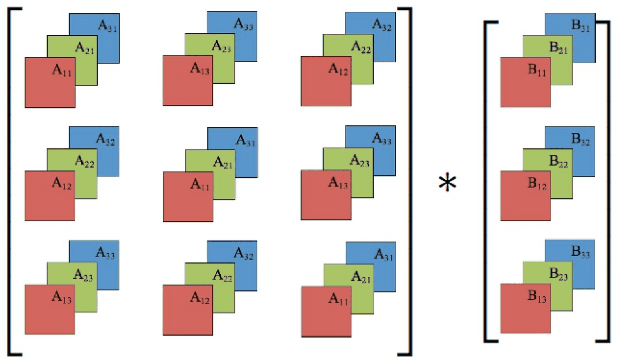
The block-circulant matrix behind the t-product, next to the stacked frontal slices of the second tensor.
There is a second way to read it. View A as an n1×n2 matrix whose entries are tubes of length n3. The t-product is then ordinary matrix multiplication, with circular convolution of tubes in place of multiplying numbers. That circularity explains both why the product is fast and where its main assumption hides.
Written with bcirc, the product looks expensive: the block-circulant matrix has n3 times as many entries as the tensor, and the direct product costs O(n1n2l n3²). But the discrete Fourier transform diagonalizes circulant matrices and block-diagonalizes block-circulant ones. So you take an FFT of both tensors along the third mode, multiply matching frontal slices as n3 independent matrix products, and take an inverse FFT. The transforms cost O((n1n2 + n2l + n1l) n3 log n3), the slice products O(n1n2l n3) in total, and the products can run in parallel. For real data the Fourier slices come in complex-conjugate pairs, so only about half of them need computing.
Transpose, identity and orthogonality
- The t-transpose AT, of size n2×n1×n3, transposes every frontal slice and then reverses the order of slices 2 to n3.
- The identity tensor has the identity matrix as its first frontal slice and zeros everywhere else.
- A tensor Q is orthogonal when QT ∗ Q = Q ∗ QT = I.
- A tensor is f-diagonal when every frontal slice is a diagonal matrix.
The decomposition
Every real n1×n2×n3 tensor can be written as A = U ∗ S ∗ VT, with U (n1×n1×n3) and V (n2×n2×n3) orthogonal and S (n1×n2×n3) f-diagonal. The diagonal tubes of S, the singular tubes, take the place of singular values, and the lateral slices of U and V take the place of singular vectors. The recipe is short:
- Take the FFT of A along the third mode.
- Compute an ordinary matrix SVD of every frontal slice.
- Take the inverse FFT of the stacked factors.
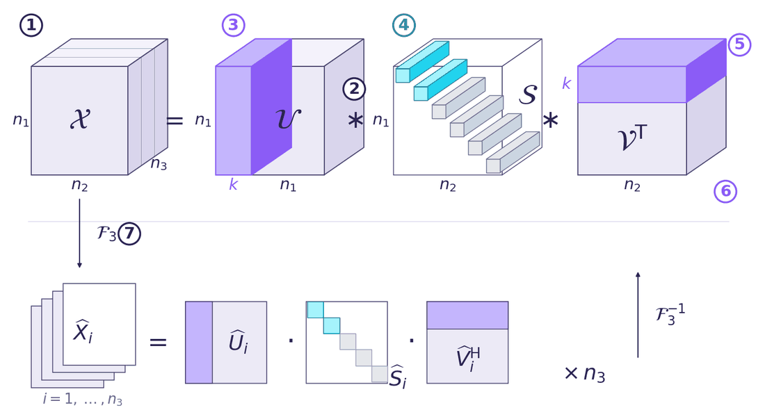
t-SVD of an n1×n2×n3 tensor. The coloured parts are what a rank-k truncation keeps; the bottom row is the same factorization as one matrix SVD per frontal slice after a transform along the third mode.
Truncation and tubal rank
As with matrices, you can keep only the first k lateral slices of U and V and the first k singular tubes:
Ak = Uk ∗ Sk ∗ VkT = ∑i=1..k U(:, i, :) ∗ S(i, i, :) ∗ V(:, i, :)T
Kilmer and Martin showed that Ak is the best approximation of A in the Frobenius norm among all tensors of tubal rank at most k, where the tubal rank is the number of non-zero singular tubes. It is the t-product counterpart of the Eckart–Young theorem. The guarantee lives inside this algebra and says nothing about CP rank or Tucker rank. Computationally, truncation just means keeping the k largest singular values in every Fourier-domain slice.
This property is what makes t-SVD useful for learning and not only for compression. In my thesis each training image was one lateral slice, and the first k lateral slices of U became the basis that images were projected onto before classification.
Cost
A full t-SVD costs n3 independent SVDs of n1×n2 matrices plus the transforms along the third mode, which take O(n1n2n3 log n3). For real input only ⌊n3/2⌋ + 1 of those SVDs are needed, because the rest are complex conjugates. The block-circulant matrix is never formed, and the slice SVDs parallelize trivially.
A NumPy sketch
This version returns economy-size factors and takes an optional truncation rank k. The only subtle part is the second loop: for real input the factors have to respect the conjugate pairs, or the inverse FFT will not come back real.
import numpy as np

def t_product(A, B):
    Af, Bf = np.fft.fft(A, axis=2), np.fft.fft(B, axis=2)
    Cf = np.einsum("ijk,jlk->ilk", Af, Bf)   # one product per slice
    return np.real(np.fft.ifft(Cf, axis=2))

def t_transpose(A):
    At = np.transpose(A, (1, 0, 2))          # transpose each slice
    return np.concatenate([At[:, :, :1], At[:, :, :0:-1]], axis=2)

def t_svd(A, k=None):
    n1, n2, n3 = A.shape
    r = min(n1, n2) if k is None else k
    Af = np.fft.fft(A, axis=2)
    Uf = np.zeros((n1, r, n3), complex)
    Sf = np.zeros((r, r, n3), complex)
    Vf = np.zeros((n2, r, n3), complex)
    half = n3 // 2 + 1
    for i in range(half):                    # SVD of each Fourier slice
        u, s, vh = np.linalg.svd(Af[:, :, i], full_matrices=False)
        Uf[:, :, i] = u[:, :r]
        Sf[:, :, i] = np.diag(s[:r])
        Vf[:, :, i] = vh[:r].conj().T
    for i in range(half, n3):                # real input: conjugate pairs
        Uf[:, :, i] = Uf[:, :, n3 - i].conj()
        Sf[:, :, i] = Sf[:, :, n3 - i].conj()
        Vf[:, :, i] = Vf[:, :, n3 - i].conj()
    back = lambda T: np.real(np.fft.ifft(T, axis=2))
    return back(Uf), back(Sf), back(Vf)

A = np.random.rand(6, 5, 4)
U, S, V = t_svd(A)
print(np.allclose(A, t_product(t_product(U, S), t_transpose(V))))  # True

U2, S2, V2 = t_svd(A, k=2)                   # tubal rank 2
A2 = t_product(t_product(U2, S2), t_transpose(V2))
print(np.linalg.norm(A - A2) / np.linalg.norm(A))  # relative error
The assumption hidden in the FFT
The circulant structure encodes a choice: the third mode wraps around, so the last frontal slice is treated as the neighbour of the first. For some data that is harmless. For images, signals and time series it is like assuming the right edge of a photo continues from its left edge. The result also depends on which mode you put third and on the order of the slices, because t-SVD is not symmetric in its modes. My own variant, tc-SVD, keeps everything above but replaces the wrap-around with a mirror and the FFT with the DCT.
The comparison guide sets t-SVD against CP and Tucker. Part 1 of Tensor Notes starts the longer series, and the later parts are listed in the Tensor section.
Frequently asked questions
Who introduced t-SVD?
t-SVD and the t-product were introduced by Kilmer and Martin in 2011. Their work also showed that truncating the t-SVD gives the best Frobenius-norm approximation of a given tubal rank.
What does f-diagonal mean?
A tensor is f-diagonal when every frontal slice is a diagonal matrix. In t-SVD the middle factor S is f-diagonal, and its diagonal tubes, the singular tubes, play the role of singular values.
Why is t-SVD computed with the FFT?
The t-product is built from block-circulant matrices, and the discrete Fourier transform block-diagonalizes them. After an FFT along the third mode, the tensor problem splits into independent matrix SVDs, one per frontal slice.
Is truncated t-SVD optimal?
Yes, in the t-product sense: keeping k singular tubes gives the best Frobenius-norm approximation among tensors of tubal rank at most k. The guarantee does not cover CP rank or Tucker rank.
What is the tubal rank of a tensor?
The tubal rank is the number of non-zero singular tubes in the t-SVD of a tensor. It plays the role that matrix rank plays for the ordinary SVD.