
 Mahdi Molavi
In data science and machine learning, a tensor is a multi-dimensional array of numbers. The number of dimensions is its order and each dimension is a mode: a vector is a first-order tensor, a matrix is second-order, and a grayscale video (height × width × frames) is third-order. Working with the tensor directly, instead of flattening it into one long vector, keeps the structure that links neighbouring values.
Order and modes
In mathematics and physics the word carries more machinery: a tensor there also comes with rules for how it changes under a change of coordinates. For data work you can set that aside and treat a tensor of order N as an array with N indices, of size I1×I2×…×IN. A single number has order zero.
A concrete case: a thirty-second grayscale clip at 25 frames per second and 768×576 pixels is a 576×768×750 tensor. Mode 1 is height, mode 2 is width, mode 3 is time, and each of the 750 frames holds 442,368 numbers. Keep the colour channels and the same clip becomes a fourth-order tensor.
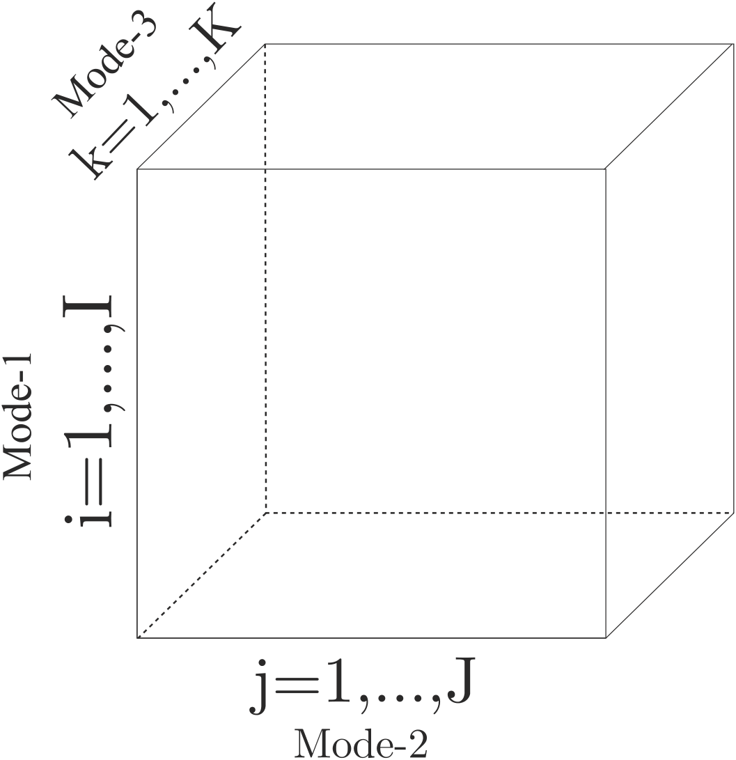
A third-order tensor and its three modes.
Fibers
Fix every index except one and you get a fiber, which is a vector. A third-order tensor X has three kinds: column fibers X(:, j, k) along mode 1, row fibers X(i, :, k) along mode 2, and tube fibers X(i, j, :) along mode 3. In the video, a tube fiber is one pixel followed through time, which is exactly the relation that flattening scatters.
Slices
Fix every index except two and you get a slice, which is a matrix. Frontal slices X(:, :, k) are the natural ones for video, since each one is a frame. Horizontal slices X(i, :, :) and lateral slices X(:, j, :) cut the same block of data from the other two directions.
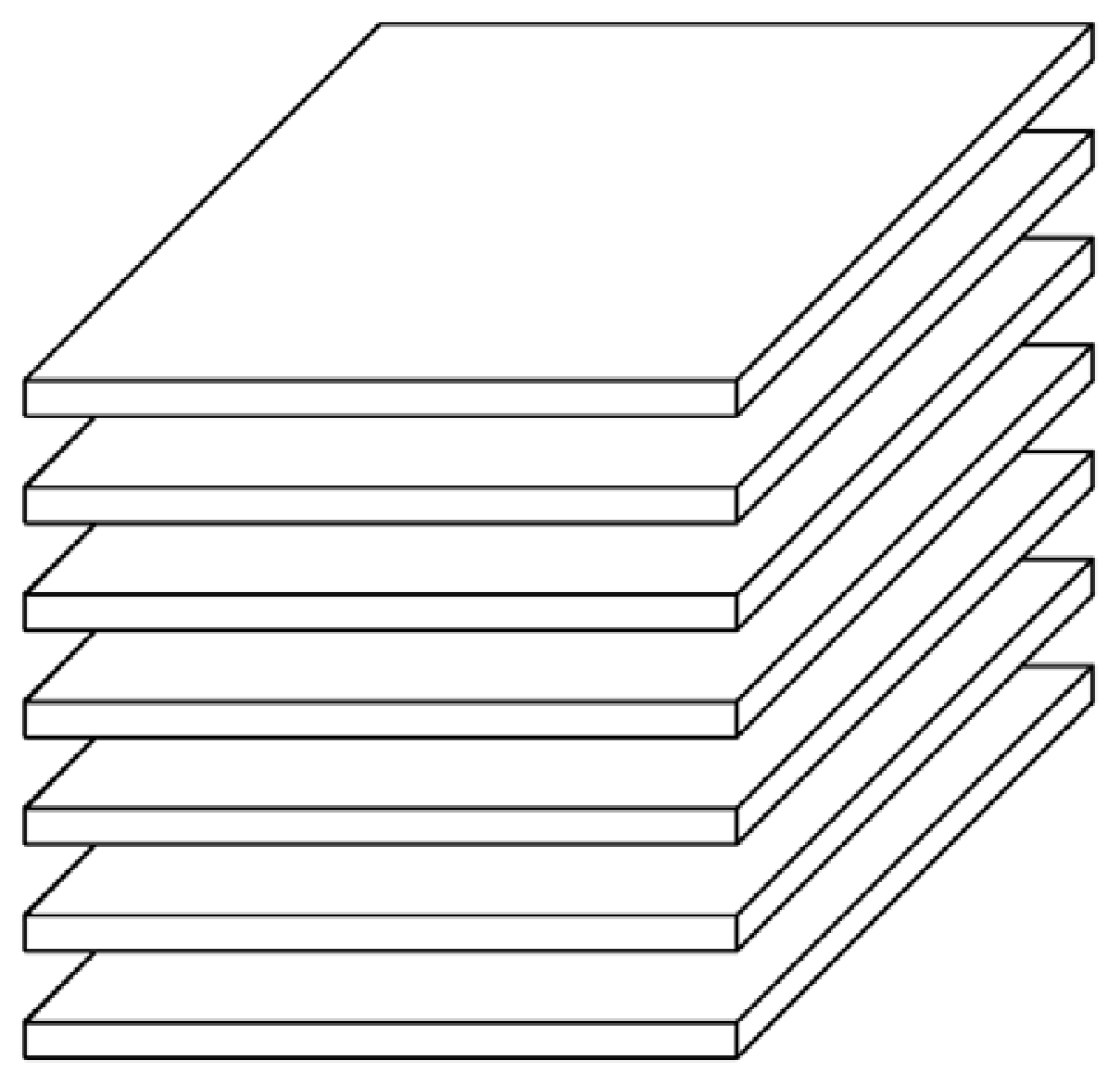
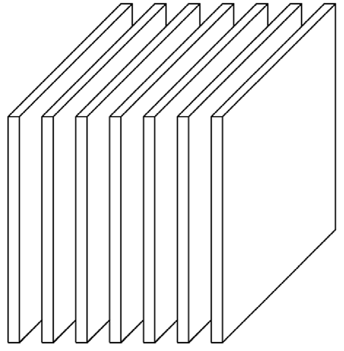
Horizontal slices (left) and lateral slices (right) of the same tensor.
Lateral slices come back later. When I classified images with t-SVD and tc-SVD in my thesis, each image was stored as one lateral slice of size n1×1×n3, so the second mode counted the samples and every image kept its two-dimensional shape.
Unfolding (matricization)
Unfolding, also called matricization, arranges the mode-n fibers of a tensor as the columns of a matrix, written X(n). For an I1×I2×I3 tensor, X(1) is I1×I2I3, X(2) is I2×I1I3 and X(3) is I3×I1I2. A 3×4×2 tensor unfolded along mode 1 becomes a 3×8 matrix, its two frontal slices side by side; along mode 2 it becomes a 4×6 matrix made of the transposed slices.
Nothing is thrown away. Each unfolding is another view of the same numbers, and it is how tensor methods hand work to matrix tools you already trust, such as the SVD. In NumPy, with n counted from 0, one common convention is np.moveaxis(X, n, 0).reshape(X.shape[n], -1, order="F"). Libraries order the columns differently, so check the convention before you compare results across codebases.
The mode-n product
The mode-n product multiplies every mode-n fiber of a tensor by the same matrix. For a tensor X of size I1×…×IN and a matrix U of size J×In, the result Y = X ×n U has the same size except that In becomes J. In unfolded form it is a single matrix product:
Y(n) = U X(n)
If J is smaller than In, mode n shrinks and the other modes are untouched; in my thesis the illustration reduces mode 2 of a tensor from 8 to 2. When the rows of U are orthonormal, every mode-n fiber is projected onto J directions, the tensor counterpart of projecting data onto principal components. The Tucker decomposition and HOSVD are built from this one operation.
Why not just flatten?
Flattening a tensor into vectors costs you in two separate ways.
- Structure. Two pixels that sit next to each other in an image can end up hundreds of positions apart in the vector, and the same pixel in consecutive frames ends up further still. The model then has to rediscover relations the array handed you for free.
- Dimension. Long vectors mean a large feature space. With a fixed number of training samples, adding features beyond a point makes predictions worse: the Hughes phenomenon (1968), one face of what Bellman called the curse of dimensionality. Compute costs grow with it. Training a kernel SVM costs roughly O(m³) time and O(m²) memory for m samples, and PCA or linear regression cost about O(mn² + n³) for n features.
Keeping data as a tensor preserves its structure, but on its own it saves nothing. The savings come from decomposing the tensor, the way the SVD decomposes a matrix, and keeping only the parts that carry information.
Where to go next
The comparison of CP, Tucker and t-SVD shows what each decomposition does with these building blocks, and the t-SVD guide explains the one my thesis built on. For a longer walk through the same material, with the video example and NumPy code for unfolding and the mode-n product, read part 1 of Tensor Notes, Stop Flattening Your Data.
Frequently asked questions
Is a tensor the same as a multi-dimensional array?
For data science and machine learning, yes: a tensor is an array with N indices, and N is its order. In mathematics and physics the word also implies rules for how the object changes under a change of coordinates.
What is the difference between a fiber and a slice?
A fiber fixes every index but one, so it is a vector, such as one pixel followed through all frames of a video. A slice fixes every index but two, so it is a matrix, such as one frame.
What does unfolding (matricization) a tensor mean?
Unfolding arranges the mode-n fibers of a tensor as the columns of a matrix. No values are lost, and the result can be passed to matrix tools such as the SVD.
What is the mode-n product?
It multiplies every mode-n fiber of a tensor by the same matrix U, which in unfolded form is the single product U times X(n). It changes the size of one mode, leaves the others alone, and is the building block of the Tucker decomposition.
Why not flatten images or video into vectors?
Flattening separates values that belong together, such as neighbouring pixels or the same pixel across frames, and it inflates the feature space. Tensor methods keep that structure and give more compact features.