Tensor Notes 1: Stop Flattening Your Data

Take a thirty-second grayscale video clip at 25 frames per second and 768×576 pixels. That is 750 frames, and each frame is a grid of 442,368 numbers. Before most machine learning libraries will touch it, the standard recipe asks you to turn every frame, or the whole clip, into one long vector.

It works, in the sense that the code runs, but the geometry of the data is lost on the way. Two pixels that sit next to each other in the picture can end up hundreds of positions apart in the vector. The same pixel in two consecutive frames ends up even further apart. The model now has to rediscover structure that the data handed you for free.

That frustration is where my M.Sc. research at Tarbiat Modares University started: how do you learn from large data sets without flattening them first? The answer I worked with is the tensor. This note is the first of a short series based on my thesis, and it covers the basics you need for the rest.

Why flattening hurts

There are two separate problems, and it helps to keep them apart.

You lose structure. An image is not a bag of numbers; neighbouring pixels are strongly related, and so are neighbouring frames. Vectorizing throws that geometry away, and with it information a model could have used.

You pay for dimensions. Long vectors mean a huge feature space. With a fixed number of samples, adding features eventually makes predictions worse. This is known as the Hughes phenomenon (1968), one face of what Bellman called the curse of dimensionality. The bill arrives in memory and time as well: training a kernel SVM costs roughly O(m³) time and O(m²) memory for m samples, and PCA or linear regression cost about O(mn² + n³) for n features. With big data, neither m nor n is small.

What a tensor is (for our purposes)

Mathematicians and physicists use the word with a lot of machinery attached. For data work you can treat a tensor as a multi-dimensional array. The number of dimensions is its order, and each dimension is a mode. A single number is order zero, a vector is order one, a matrix is order two. Our grayscale clip is an order-three tensor of size 576×768×750: height, width and frames. Keep the colour channels and it becomes order four.

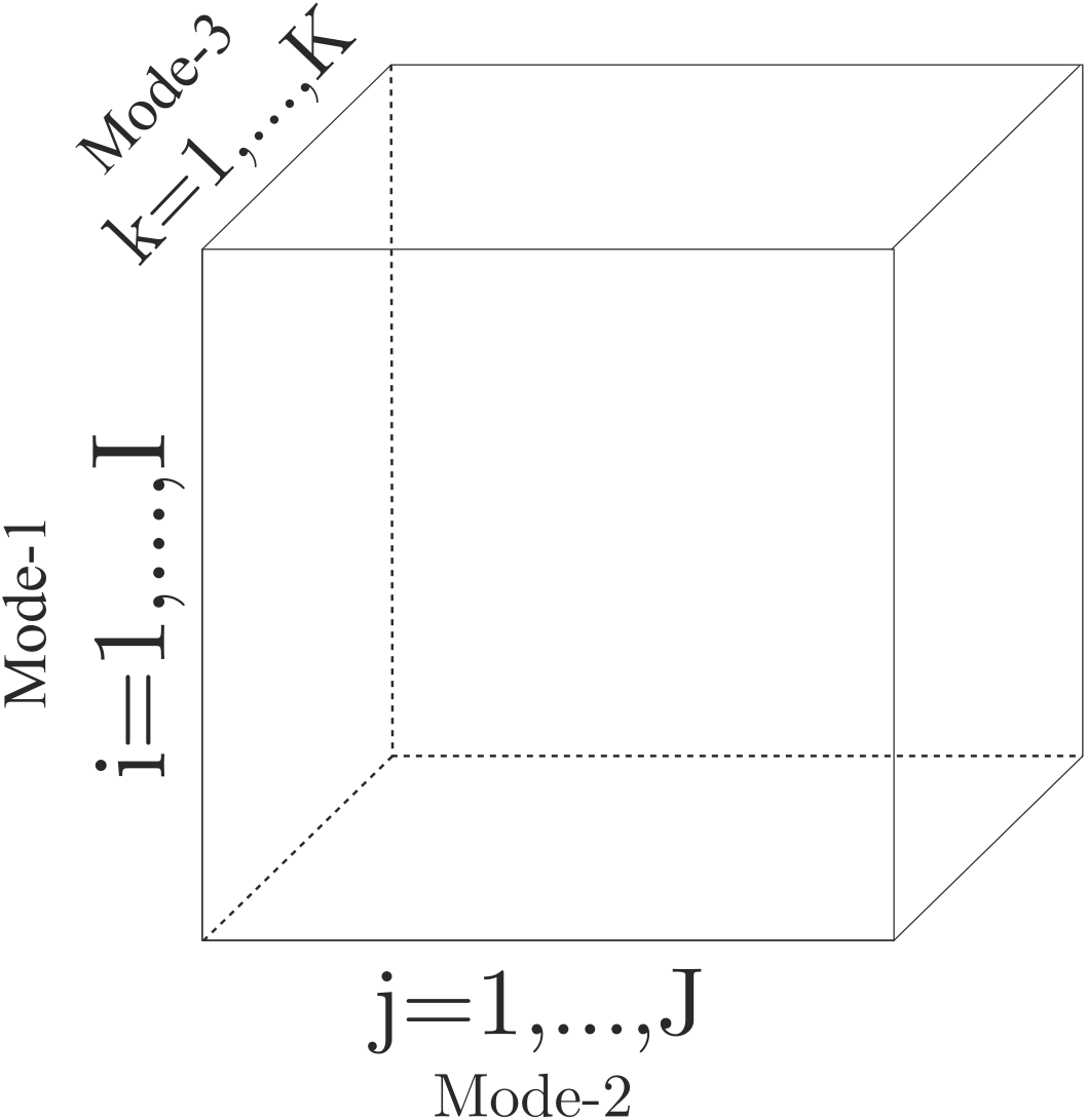
A third-order tensor and its three modes.

Fibers and slices

Two ideas make tensors easy to reason about.

A fiber is what you get when you fix every index except one. In a third-order tensor there are column fibers, row fibers and tube fibers. In the video example, a tube fiber is one pixel followed through time, which is exactly the kind of structure flattening destroys.

A slice fixes every index except two, so it is a matrix. Frontal slices are the natural ones for video: each frontal slice is one frame. Horizontal and lateral slices cut the same block of data from the other two directions.

 
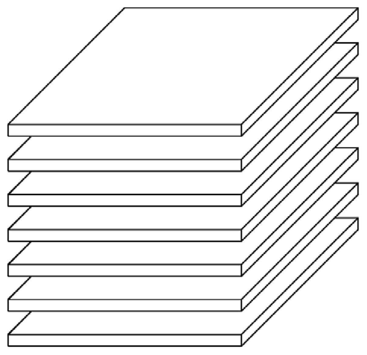
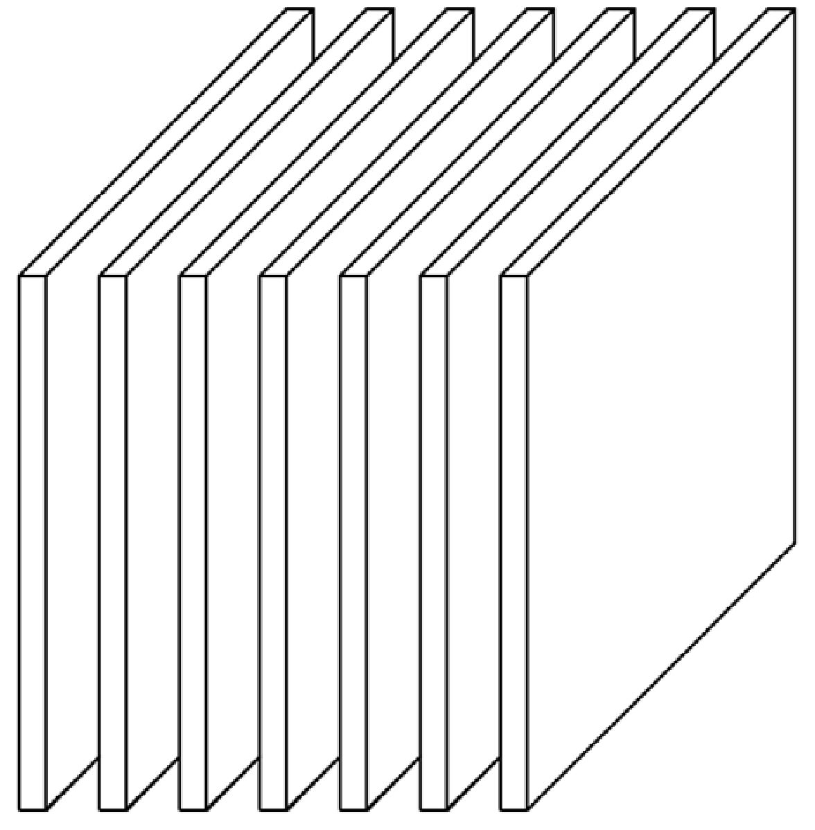
Horizontal slices (left) and lateral slices (right) of the same tensor.

Unfolding: talking to matrix algorithms

Sooner or later you want to use the matrix tools you already trust. Unfolding (also called matricization) arranges the mode-n fibers of a tensor as the columns of a matrix. A 3×4×2 tensor unfolded along mode 1 becomes a 3×8 matrix: the two frontal slices placed side by side. Unfold along mode 2 and you get the transposed slices instead. Each unfolding is just another view of the same data; nothing is thrown away.

The mode-n product: shrinking one dimension at a time

The operation I used most is the mode-n product. You multiply every mode-n fiber of the tensor by the same matrix U. If U has fewer rows than the mode has entries, that mode shrinks while the others stay untouched. In the thesis I illustrate it by reducing mode 2 of a tensor from 8 to 2. When the rows of U are orthonormal, every mode-n fiber is projected onto a few directions, which is the tensor counterpart of projecting data onto principal components. Every decomposition in this series uses it.

Here is a small NumPy version of both operations:

import numpy as np

def unfold(X, mode):
    # the mode-n fibers become the columns of a matrix
    return np.moveaxis(X, mode, 0).reshape(X.shape[mode], -1, order="F")

def mode_n_product(X, U, mode):
    # multiply every mode-n fiber of X by the matrix U
    Y = U @ unfold(X, mode)
    rest = [s for i, s in enumerate(X.shape) if i != mode]
    return np.moveaxis(Y.reshape([U.shape[0]] + rest, order="F"), 0, mode)

X = np.random.rand(3, 8, 5)
U = np.random.rand(2, 8)
print(mode_n_product(X, U, 1).shape)   # (3, 2, 5)

Where decompositions come in

Storing data as a tensor keeps its structure; the savings come from decomposing it, the way SVD decomposes a matrix, and keeping only the parts that carry information. The classic options are the CP decomposition, which writes a tensor as a sum of rank-one pieces, and the Tucker decomposition, which uses a small core tensor and one factor matrix per mode and is usually computed with the higher-order SVD (HOSVD).

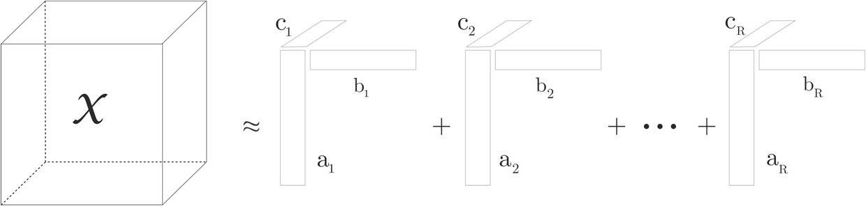
CP decomposition: a sum of R rank-one tensors.

Both are useful, but for the learning problems I cared about a third family fit better: the t-product and t-SVD, which keep the optimal truncation property of the matrix SVD. That is the subject of the next note. After that comes the part I built myself, a variant called tc-SVD that replaces the circular assumption hidden inside t-SVD with a mirror.

A first look at t-SVD

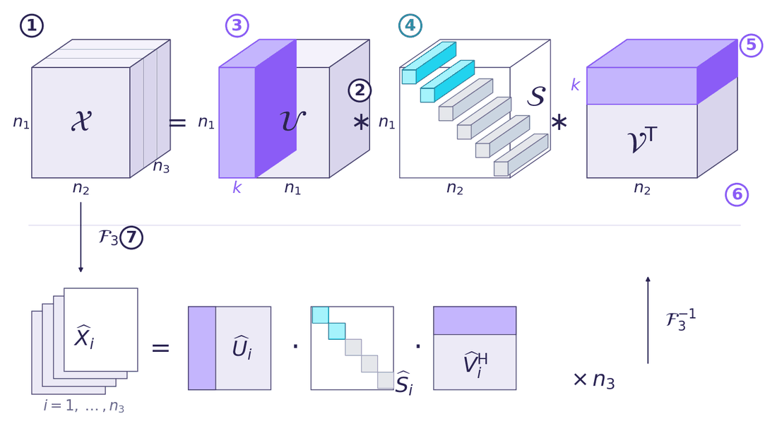
t-SVD, annotated. Violet and cyan mark what a rank-k truncation keeps; the numbers are explained below.

The next note builds this decomposition step by step, but you can already read the picture. X (1) is the data, of size n₁×n₂×n₃, and ∗ (2) is the t-product, a multiplication that works along the third mode. U (3) is orthogonal; its lateral slices act as a basis, and the violet block is the first k of them. S (4) is f-diagonal: only the tubes along its diagonal are non-zero, and the first k (cyan) are kept. V^T (5) is the t-transpose of an orthogonal V, and its violet rows pair each sample with the kept basis. Keeping only the coloured parts, k of each (6), gives X ≈ U_k ∗ S_k ∗ V_k^T. The bottom row (7) shows why the method is cheap: after an FFT along the third mode (a DCT in tc-SVD) the whole factorization is n₃ ordinary matrix SVDs, one per frontal slice.

This series is based on my M.Sc. thesis, “Big Data Learning with Tensor Representation”, supervised by Dr. Mansoor Rezghi at Tarbiat Modares University. A short summary of the thesis is here.

This note is also available in Persian: read the Persian version.