 Mahdi Molavi
tc-SVD is a singular value decomposition for third-order tensors built on a cosine-transform tensor product, the tc-product. It replaces the periodic (wrap-around) boundary hidden in t-SVD with a reflective (mirror) boundary, so the discrete cosine transform (DCT) takes the place of the FFT and every computation stays in real numbers. It was developed in Mahdi Molavi's M.Sc. thesis at Tarbiat Modares University; a closely related cosine-transform product appears in Kernfeld, Kilmer and Aeron (2015).
The assumption it removes
The t-product behind t-SVD is a circular convolution along the third mode. Image deblurring shows why that matters. A blurred pixel is a weighted sum of its neighbours, yi = ∑j hi−j xj, and near the edge of the image that sum needs pixels outside the picture. You have to assume something about them, and that assumption is the boundary condition.
The periodic boundary pretends the signal repeats: whatever falls off the right edge comes back in from the left. The blur becomes a circulant matrix, and the FFT makes every computation with it fast. The t-product applies exactly this model along the third mode of a tensor. The trouble is that real data is rarely periodic. The right edge of a photo has nothing to do with its left edge, and the end of a time series usually has nothing to do with its start. Gluing them together creates a jump that was never in the data, and in image restoration the periodic boundary typically leaves artifacts along the edges. Ng, Chan and Tang (1999) showed that a reflective boundary gives better restorations at the same O(n log n) cost.
A mirror instead of a wrap
A reflective boundary assumes the signal continues as its own mirror image: the value just outside the edge equals the value just inside it, so there is no artificial jump. The blur matrix is then Toeplitz-plus-Hankel instead of circulant, and for symmetric kernels matrices of this form are diagonalized by the DCT, which also runs in O(n log n).
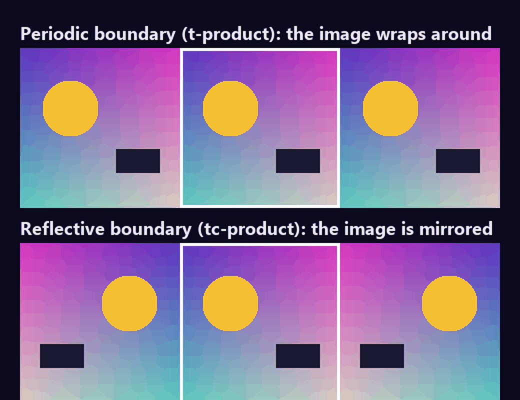
The same picture (framed) padded two ways. The periodic boundary glues mismatched edges together; the reflective one continues smoothly.
The tc-product and tc-SVD
In the thesis I carried this idea over to tensors. Instead of a block-circulant matrix, the frontal slices go into a block Toeplitz-plus-Hankel matrix, and the DCT along the third mode block-diagonalizes it. The tc-product of two tensors takes three steps:
- transform both tensors along the third mode with a DCT-based transform (the DCT plus a diagonal scaling and a shift that match the Toeplitz-plus-Hankel structure);
- multiply their frontal slices pairwise, as ordinary matrices;
- transform the result back.
The product keeps what linear algebra needs. It is linear and associative, it has an identity and a transpose, and orthogonal tensors exist. With the DCT in its orthonormal form, multiplying by an orthogonal tensor also preserves the Frobenius norm. The decomposition then follows the t-SVD pattern:
A = U ∗c S ∗c VT
with orthogonal U and V and f-diagonal S. You take the DCT along the third mode, run an ordinary SVD on every frontal slice and transform the factors back. With the orthonormal DCT, truncating to the first k terms gives the best Frobenius-norm approximation among tensors of rank at most k under this product, the same guarantee t-SVD has under its own.
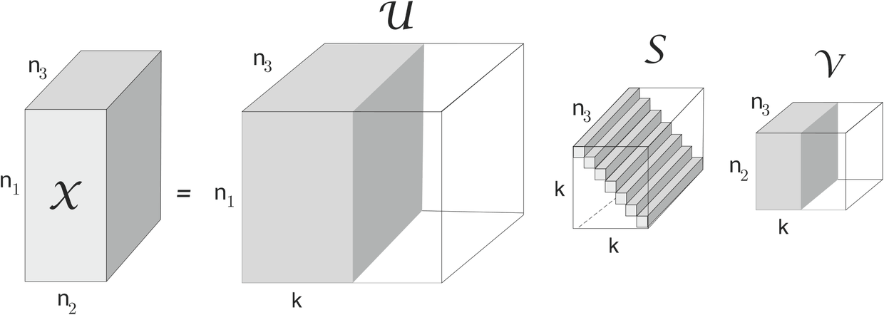
Truncated tc-SVD: only k lateral slices of U and V, and k diagonal tubes of S, are kept.
Two practical differences from t-SVD follow. There are no complex numbers and no conjugate-pair bookkeeping, and in my experiments the DCT-based versions were faster in almost every comparison, often taking about half the time. The thesis also describes a cheaper compression route that skips the full decomposition: add up all frontal slices, take one SVD of the sum, keep k1 left and k2 right singular vectors, and compress every slice into a small k1×k2 core.
What I used it for
- Classification. Each image is a lateral slice of the data tensor. Approach I generalizes the t-SVD method of Kilmer and colleagues, with one shared basis from the first k lateral slices of U. Approach II, new in the thesis, builds one tc-SVD basis per class and assigns a test image to the class that reconstructs it with the smallest residual. Tested on MNIST and the CBCL face set.
- Clustering. k-means on a truncated V, optionally reduced from both sides (two-sided truncation), on ORL, PIE-pose, Extended Yale B and COIL-100.
- fMRI. Telling early mild cognitive impairment (eMCI) apart from healthy controls with resting-state fMRI from ADNI (82 subjects), each subject stored as a matrix of 130 time points by 90 brain regions.
- Streaming data. An incremental tc-SVD that generalizes Brand's incremental SVD (2002): new slices are transformed and every frontal slice is updated instead of recomputed.
Results, as reported
- On MNIST and CBCL, accuracy was almost exactly that of t-SVD (both MNIST curves sit around 97%), in roughly half the run time.
- In clustering (best NMI, averaged over ten runs), two-sided tc-SVD was best on ORL (0.730) and Extended Yale B (0.799). On PIE-pose every t-SVD and tc-SVD variant was close to perfect, with two-sided t-SVD slightly ahead (0.994). On COIL-100, HOSVD (0.749) and NMF (0.730) beat both tensor SVDs.
- One-sided tc-SVD was faster than one-sided t-SVD on every data set: it needed less than half the time on ORL, Yale B and COIL-100, and the gap on PIE-pose was about 13%. HOSVD was faster still on Yale B and COIL-100.
- For eMCI against healthy controls (82 subjects, leave-one-out), the best accuracy over k was 86.5% for tc-SVD (k = 44) against 70.7% for t-SVD (k = 13), the largest gap in the thesis. The tc-SVD figure was sensitive to k, and this is a small-study research result, not a diagnostic tool.
So the mirror boundary is not a universal winner. Its consistent advantage was speed, and the accuracy gains depended on the data set.
Code
The MATLAB implementation is open source at github.com/mahdipc/tcSVD under the MIT License. Besides tc-SVD it has the FFT-based t-SVD for comparison, incremental updates, the classification and clustering code and an HOSVD baseline. It needs the Tensor Toolbox for MATLAB. Function names below are spelled as in the repository:
A = rand(32, 50, 32);           % 50 images of 32x32, one lateral slice each
[U, S, V] = tcSVD(A, 10);       % rank-10 tc-SVD
Ak = tcProdact(U, tcProdact(S, tcTranspose(V)));
relative_error = norm(A(:) - Ak(:)) / norm(A(:))
Part 3 of Tensor Notes (see the Tensor section) has a NumPy and SciPy sketch, and the thesis summary covers the whole project.
Frequently asked questions
What is the difference between t-SVD and tc-SVD?
Both transform the tensor along the third mode, run one matrix SVD per frontal slice and transform back. t-SVD uses the FFT, assumes a periodic boundary and works in complex arithmetic; tc-SVD uses the DCT, assumes a reflective boundary and stays in real numbers.
Is tc-SVD always better than t-SVD?
No. In the thesis experiments it matched t-SVD on classification accuracy, gave better clusters on ORL and Extended Yale B and reached a higher best accuracy on a small fMRI study of early Alzheimer's (86.5% against 70.7%, a figure that was sensitive to k). t-SVD was slightly ahead on PIE-pose, and HOSVD and NMF beat both on COIL-100. It was faster than t-SVD in almost every comparison.
Why is tc-SVD faster than t-SVD?
The DCT keeps every computation in real numbers, while the FFT works with complex numbers even when the data is real. In the thesis experiments the DCT-based versions were faster in almost every comparison and often took about half the time.
Who developed tc-SVD?
tc-SVD and the learning methods built on it come from Mahdi Molavi's M.Sc. thesis, Big Data Learning with Tensor Representation, Tarbiat Modares University (2019), supervised by Dr. Mansoor Rezghi. A closely related cosine-transform product appears in Kernfeld, Kilmer and Aeron (2015).
Is there code for tc-SVD?
Yes. A MATLAB implementation with classification, clustering and incremental updates is at github.com/mahdipc/tcSVD under the MIT License.