

A decomposition is only interesting if it helps you do something. In this note I use tc-SVD, the mirror-boundary decomposition from part three, for two everyday machine learning jobs: classifying images and clustering them. I will show the numbers from my thesis as they are, including the cases where tc-SVD did not win.
How images become a tensor
Each image is an n1×n3 matrix. Instead of flattening it into a vector, I subtract the mean image and stand the result on its side as a lateral slice of a tensor, an n1×1×n3 block. Put all training images next to each other and you get one n1×m×n3 tensor, with one lateral slice per image. The image keeps its two-dimensional shape the whole time.
Two ways to classify
Approach I follows the method Kilmer and colleagues proposed for t-SVD, and I generalized it to tc-SVD. Decompose the training tensor, keep the first k lateral slices of U, and use them as a basis. Every training image and every test image is projected onto that basis, which gives a small k×1×n3 coefficient slice for each one. A test image is then compared with the training coefficients. A nice sanity check: if the images have only one column (n3 = 1), this reduces exactly to classic PCA.
Approach II is new in the thesis. Instead of one shared basis, it builds a separate tc-SVD basis Ui for every class. To classify a test image, you try to rebuild it from each class's basis and measure what is left over:
label = argmini ‖ B − Ui ∗c UiT ∗c B ‖
The class whose basis explains the image best, with the smallest residual, wins. It is simple, it needs no training beyond the decompositions, and adding a new class means computing one more basis without touching the others.
Classification results
I tested on two standard data sets. MNIST has 70,000 handwritten digits of 28×28 pixels, 10,000 of them held out for testing. CBCL (from MIT) is a face-detection set of 19×19 images: 2,429 faces and 4,548 non-faces for training, and 472 faces and 23,573 non-faces for testing.
On accuracy, tc-SVD landed almost exactly where Kilmer's t-SVD method did. The two differed in speed: because the DCT keeps everything in real numbers, the tc-SVD versions took roughly half the time.
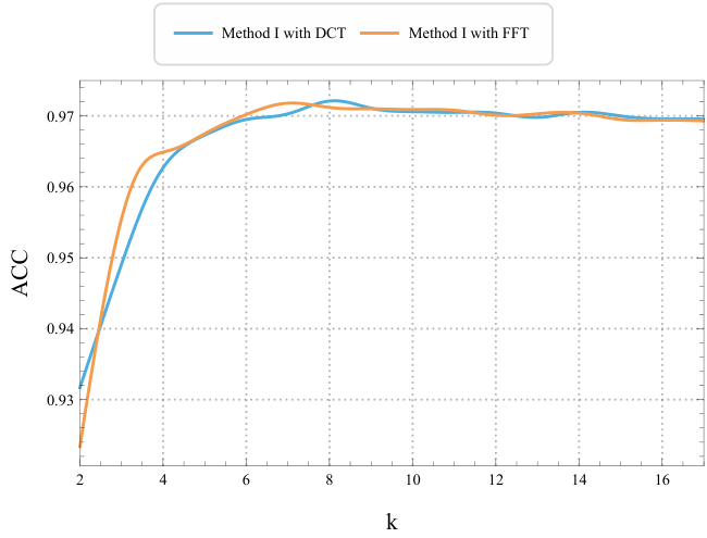
MNIST accuracy against k, the number of kept slices: the DCT (tc-SVD) and FFT (t-SVD) curves sit on top of each other, around 97%.
The per-digit error rates show where the difficulty is. With k = 7 kept slices, the digit 1 was misclassified only 0.53% of the time, and 0 only 0.82%. The hardest digits were 8 (4.6%), 4 and 7 (4.4% each) and 3 (3.8%). Averaged over the ten digits, that is an error rate of about 2.8%. Beyond k of roughly 7 or 8, adding more slices did not help; the extra slices carry little new information.
Clustering: squeezing the data from both sides
For clustering there are no labels, so the goal is to find a small representation where k-means works well. In a tc-SVD of the data tensor, U and S are shared by all samples, and each sample's own information lives in V. So I keep a truncated V as the feature tensor.
k-means is known to struggle in high dimensions, so I added a second step: permute V and apply tc-SVD to it again, reducing the other direction as well. I call this two-sided truncation. The final features are small in both directions, and k-means runs on those.
I compared it against t-SVD (with the same one- and two-sided variants), NMF and HOSVD on four image collections:
- ORL: 400 face images of 40 people, 64×64
- PIE-pose: 2,856 images of 68 people, 32×32
- Extended Yale B (subset): 1,710 images of 38 people, 192×168
- COIL-100: 7,200 images of 100 objects, 128×128
Here is the best NMI (normalized mutual information, higher is better) each method reached, averaged over ten runs:
| Method | ORL | PIE-pose | Yale B | COIL-100 |
|---|---|---|---|---|
| tc-SVD | 0.670 | 0.986 | 0.784 | 0.621 |
| tc-SVD, two-sided | 0.730 | 0.973 | 0.799 | 0.680 |
| t-SVD | 0.605 | 0.983 | 0.670 | 0.593 |
| t-SVD, two-sided | 0.636 | 0.994 | 0.756 | 0.583 |
| NMF | 0.694 | 0.847 | 0.636 | 0.730 |
| HOSVD | 0.706 | 0.909 | 0.756 | 0.749 |
Two-sided tc-SVD gave the best result on ORL and Yale B. On PIE-pose all the t-SVD and tc-SVD variants were close to perfect, with two-sided t-SVD slightly ahead. On COIL-100, HOSVD and NMF did better, so the mirror boundary is not a universal winner.
One-sided tc-SVD was faster than one-sided t-SVD on every data set. On ORL, Yale B and COIL-100 it needed less than half the time (24.9 against 58.7 on Yale B and 24.8 against 62.3 on COIL-100, in the run-time units the thesis reports). On PIE-pose the gap was about 13%, and there the two-sided tc-SVD was actually slower than two-sided t-SVD. HOSVD was faster still on Yale B and COIL-100 (21.1 and 15.1), and NMF needed 1,225 on COIL-100.
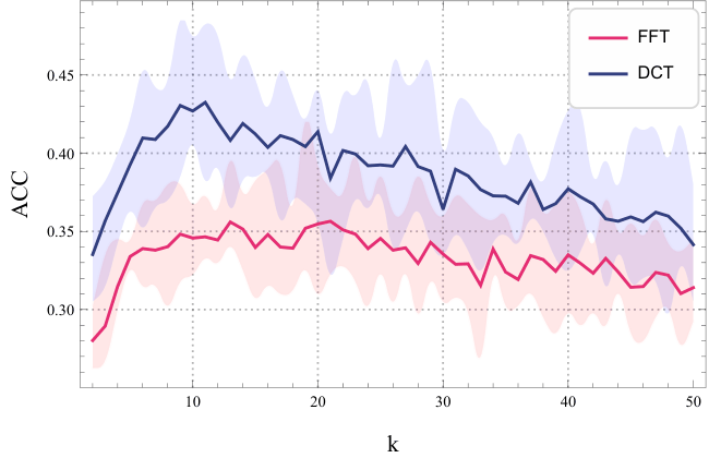
Clustering accuracy on ORL for different k: DCT (tc-SVD) stays above FFT (t-SVD) across the range. Shaded bands show the spread over runs.
What I take from it
In these experiments tc-SVD matched or beat t-SVD on accuracy in most cases and was faster in almost every comparison, often by a factor of two or more. On ORL and Yale B the mirror boundary also gave clearly better clusters, while on COIL-100 neither tensor SVD reached HOSVD or NMF. For large data, a large cut in run time at the same accuracy is often the result that matters most in practice.
The last note in this series takes the method out of benchmark land: detecting early mild cognitive impairment in brain scans, and keeping a decomposition up to date when data keeps arriving.
Part of a series based on my M.Sc. thesis, “Big Data Learning with Tensor Representation”, supervised by Dr. Mansoor Rezghi at Tarbiat Modares University.
This note is also available in Persian: read the Persian version.