Tensor Notes 3: tc-SVD, a Tensor SVD with a Mirror Boundary

In the last note I ended on a small complaint about t-SVD: its block-circulant structure assumes the third dimension wraps around, so the last slice is treated as the neighbour of the first. This note is about what I did with that complaint. The result is a tensor product built on the cosine transform, which I call the tc-product, and a decomposition built on it, tc-SVD. A closely related cosine-transform product appears in Kernfeld, Kilmer and Aeron (2015). What the thesis adds is the learning side: compression, classification, clustering and a streaming update built on tc-SVD, together with the experiments behind them.

The t-product is a convolution in disguise

The easiest way to see the problem is through image deblurring, where the same mathematics shows up. A blurred pixel is a weighted sum of its neighbours: y_i = Σ h_i−j x_j, where h is the blur kernel. Near the edge of the image, that sum needs pixels that lie outside the picture. We do not have them, so we have to assume something. That assumption is called the boundary condition.

The simplest choice is the periodic boundary: pretend the image repeats, so whatever falls off the right edge comes back in from the left. The blur then becomes a circulant matrix, and the FFT solves everything quickly. The t-product is exactly this model applied along the third mode of a tensor, which is why the FFT made it cheap in part two.

The trouble is that almost nothing in the real world is periodic. The right edge of a photo has nothing to do with its left edge, and gluing them together creates a jump that was never in the data. In image restoration the periodic boundary typically leaves artifacts along the edges. Ng, Chan and Tang (1999) showed that a reflective boundary gives better restorations at the same O(n log n) cost.

Put a mirror there instead

A reflective boundary assumes the image continues as its own mirror image. The pixel just outside the edge equals the pixel just inside it. There is no artificial jump, and for images it is a much more natural assumption.

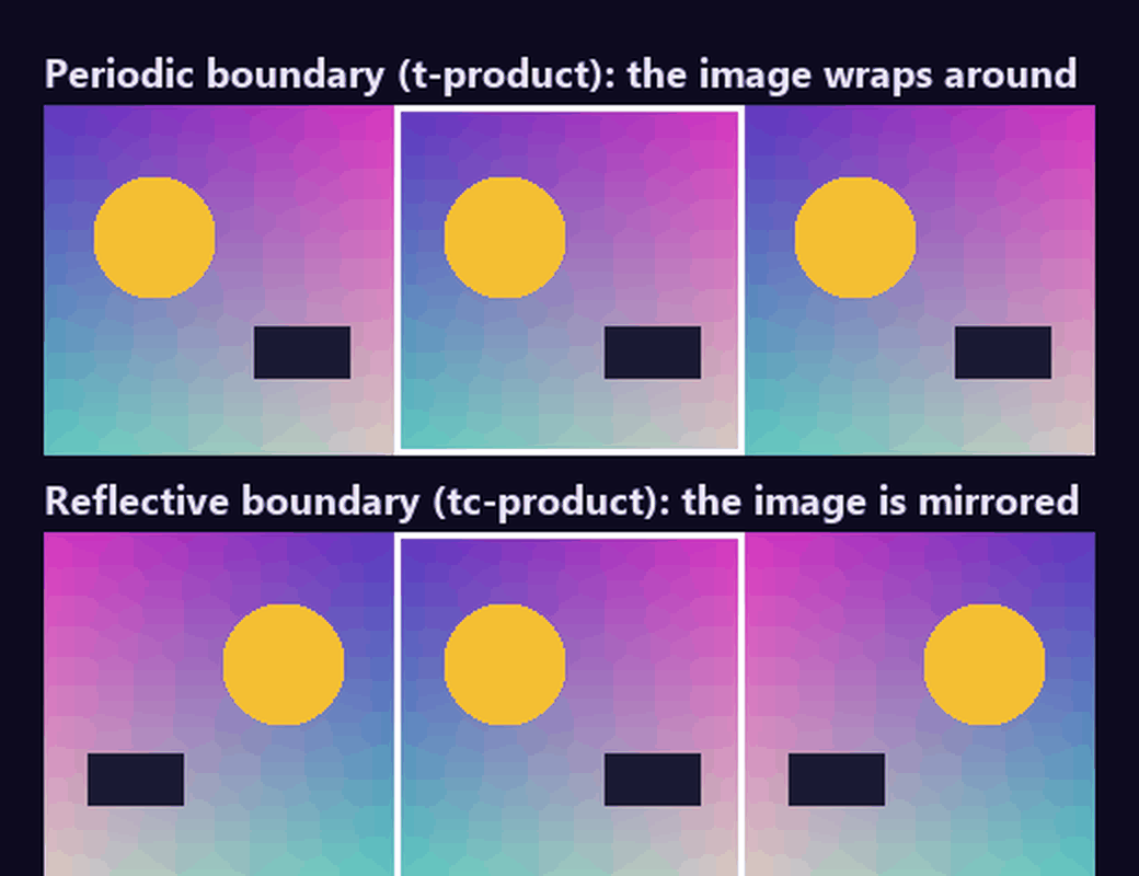
The same picture (framed) padded two ways. The periodic boundary glues mismatched edges together; the reflective one continues smoothly.

With a reflective boundary the blur matrix is no longer circulant. It becomes a Toeplitz-plus-Hankel matrix. That sounds worse, but a known result helps: for symmetric kernels, matrices of this form are diagonalized by the discrete cosine transform (DCT), just as circulant matrices are diagonalized by the FFT. The DCT also runs in O(n log n).

From one dimension to tensors: the tc-product

The thesis carries this idea over to tensors. Instead of arranging the frontal slices of a tensor into a block-circulant matrix, I arrange them into a block Toeplitz-plus-Hankel matrix, and I show that the DCT along the third mode block-diagonalizes it. The tc-product of two tensors then works like this:

1. Transform both tensors along the third mode with a DCT-based transform.
2. Multiply their frontal slices pairwise, as ordinary matrices.
3. Transform the result back.

It keeps the properties you need to do linear algebra: it is linear and associative, it has an identity and a transpose, and orthogonal tensors exist. With the DCT in its orthonormal form, multiplying by an orthogonal tensor also preserves the Frobenius norm.

There is also a practical bonus. The FFT works with complex numbers, even when your data is real. The DCT does not; everything stays real. In my experiments the DCT-based versions were faster in almost every comparison, and often took about half the time of their FFT-based counterparts.

tc-SVD

With the tc-product in place, the SVD follows the same pattern as before: A = U ∗_c S ∗_c V^T, with orthogonal U and V and an f-diagonal S. To compute it you take the DCT along the third mode, run an ordinary SVD on every frontal slice, and transform the factors back. As with t-SVD, truncating to the first k terms gives the best Frobenius-norm approximation among tensors of rank at most k under this product, which is what makes it useful for compression and learning.

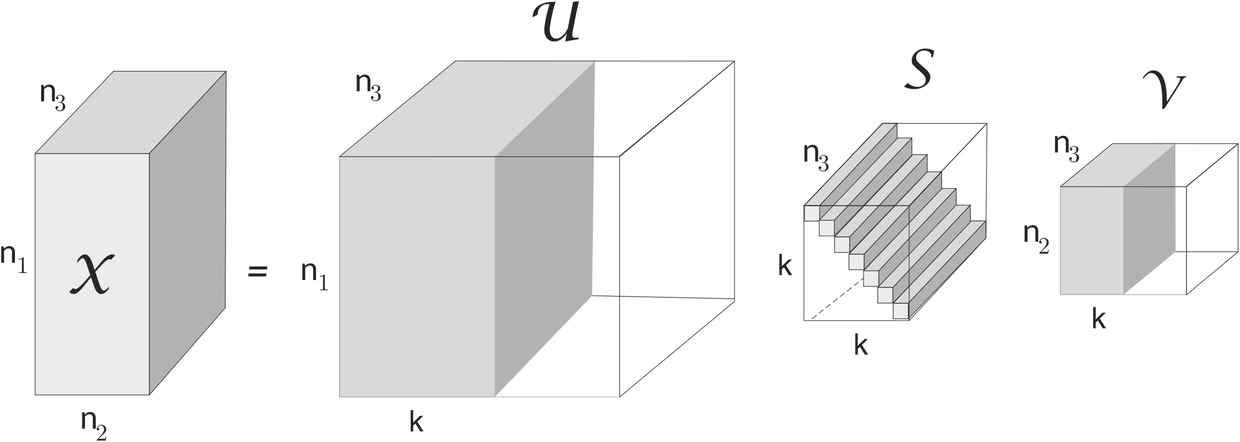
Truncated tc-SVD: only k lateral slices of U and V, and k diagonal tubes of S, are kept.

Here is a short sketch in NumPy and SciPy. To keep it readable I use the orthonormal DCT directly. The exact transform behind the Toeplitz-plus-Hankel product also adds a diagonal scaling and a shift-and-add of neighbouring slices, as in Kernfeld, Kilmer and Aeron (2015), but the shape of the algorithm is the same.

import numpy as np
from scipy.fft import dct, idct

def c_product(A, B):
    Ac = dct(A, type=2, norm="ortho", axis=2)
    Bc = dct(B, type=2, norm="ortho", axis=2)
    return idct(np.einsum("ijk,jlk->ilk", Ac, Bc), type=2, norm="ortho", axis=2)

def tc_svd(A):
    Ac = dct(A, type=2, norm="ortho", axis=2)   # real numbers only
    n1, n2, n3 = A.shape
    U, S, V = np.zeros((n1, n1, n3)), np.zeros((n1, n2, n3)), np.zeros((n2, n2, n3))
    for k in range(n3):
        u, s, vh = np.linalg.svd(Ac[:, :, k])
        U[:, :, k], V[:, :, k] = u, vh.T
        S[:len(s), :len(s), k] = np.diag(s)
    back = lambda T: idct(T, type=2, norm="ortho", axis=2)
    return back(U), back(S), back(V)

A = np.random.rand(6, 5, 4)
U, S, V = tc_svd(A)
Vt = np.transpose(V, (1, 0, 2))                 # transpose every frontal slice
print(np.allclose(A, c_product(c_product(U, S), Vt)))   # True

Compare it with the t-SVD code from part two: no complex numbers, and no conjugate bookkeeping.

A shortcut for compression

The obvious way to compress a tensor with tc-SVD is to keep only the first k terms. The thesis also describes a cheaper second approach that avoids computing the full decomposition at all. You add up all the frontal slices into one matrix, take a single SVD of that sum, and keep k₁ left and k₂ right singular vectors. Each slice is then compressed as a small k₁×k₂ core, by multiplying it by the truncated left vectors (transposed) on one side and the right vectors on the other. It works because, in this product, the sum of the slices of U ∗_c S ∗_c V^T factors neatly into the sums of the slices of U, S and V.

In the next note I will put tc-SVD to work on real tasks: classifying handwritten digits and faces, and clustering several image collections, with honest numbers against t-SVD, HOSVD and NMF.

Part of a series based on my M.Sc. thesis, “Big Data Learning with Tensor Representation”, supervised by Dr. Mansoor Rezghi at Tarbiat Modares University.

This note is also available in Persian: read the Persian version.