Tensor Notes 2: An SVD for Tensors, and the t-Product Behind It

The singular value decomposition is probably the most useful single idea in numerical linear algebra. Compression, denoising, recommendation, PCA: under the hood it is often an SVD. So when you move from matrices to tensors, the obvious question is whether there is an SVD for tensors too.

There are several, and none of them is perfect. The Tucker decomposition, computed with HOSVD, gives you orthogonal factor matrices, but its core tensor is dense, not diagonal. The CP decomposition gives you a clean sum of rank-one terms, but it is hard to compute and its factors are not orthogonal. In my thesis I built on a third option, introduced by Kilmer and Martin (2011): the t-product and the t-SVD that comes with it. What makes it attractive is that it behaves almost exactly like the matrix SVD you already know, and it is fast.

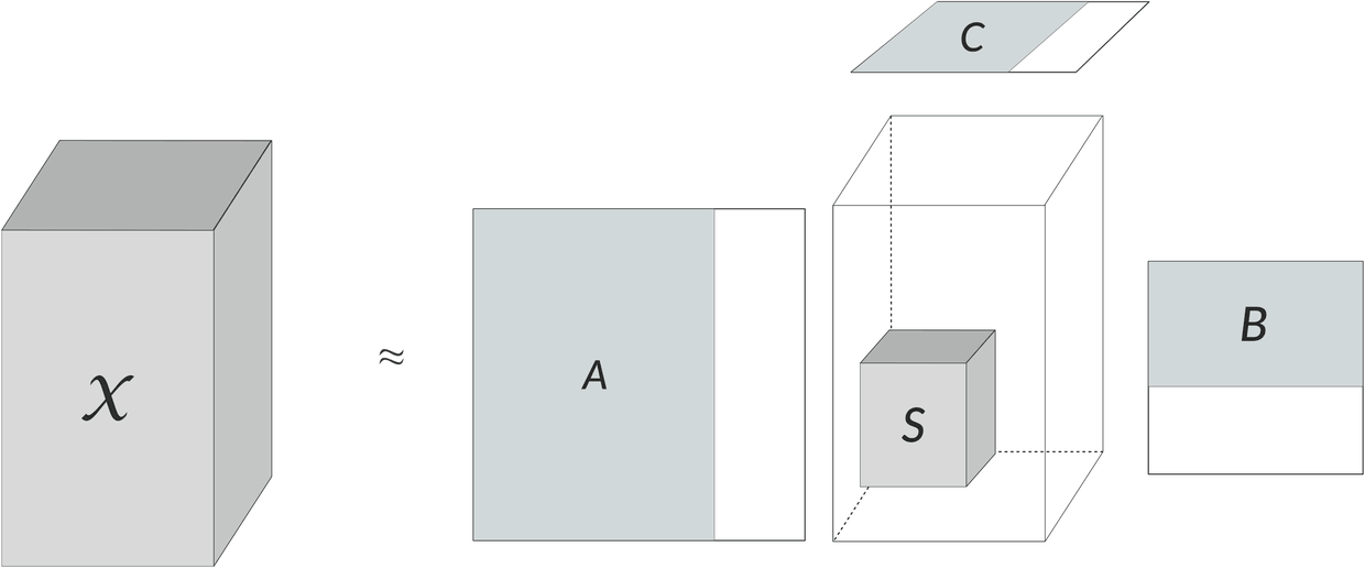
Tucker (HOSVD): orthogonal factors, but a dense core.

The t-product in one picture

Think of a third-order tensor as a stack of matrices, its frontal slices. To multiply two such stacks, the t-product builds a block-circulant matrix from the slices of the first tensor. Its first block column holds the slices in order; each following column is the previous one shifted down by one block, with the last block wrapping around to the top.

That block matrix multiplies the second tensor with its slices stacked into one tall matrix, and the result is folded back into a stack. In symbols, A ∗ B = fold(bcirc(A) · unfold(B)).

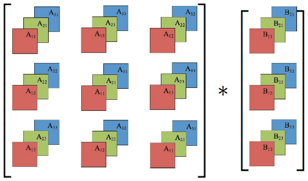
The block-circulant matrix behind the t-product.

Written like that it looks expensive. The block-circulant matrix has n₃ times as many entries as the tensor, and for a second tensor of size n₂×l×n₃ the direct product costs O(n₁n₂l n₃²).

Why it is actually cheap

Circulant matrices have a convenient property: the discrete Fourier transform diagonalizes them. For block-circulant matrices it block-diagonalizes them. So if you take an FFT along the third mode of both tensors, the t-product falls apart into n₃ ordinary, independent matrix products, one per frontal slice. An inverse FFT brings you back.

The transforms cost O((n₁n₂ + n₂l + n₁l) n₃ log n₃), the n₃ slice products cost O(n₁n₂l n₃) in total, and they can run in parallel. There is one more saving for real-valued data: the Fourier coefficients come in complex-conjugate pairs, so you only need to compute about half of the slices and fill in the rest by conjugation.

t-SVD: an SVD per slice

With the t-product in hand, the t-SVD writes a tensor as A = U ∗ S ∗ V^T, where U and V are orthogonal tensors and S is f-diagonal, meaning every frontal slice of S is a diagonal matrix. The recipe is short:

1. Take the FFT of A along the third mode.
2. Compute an ordinary SVD of every frontal slice.
3. Take the inverse FFT of the factors.

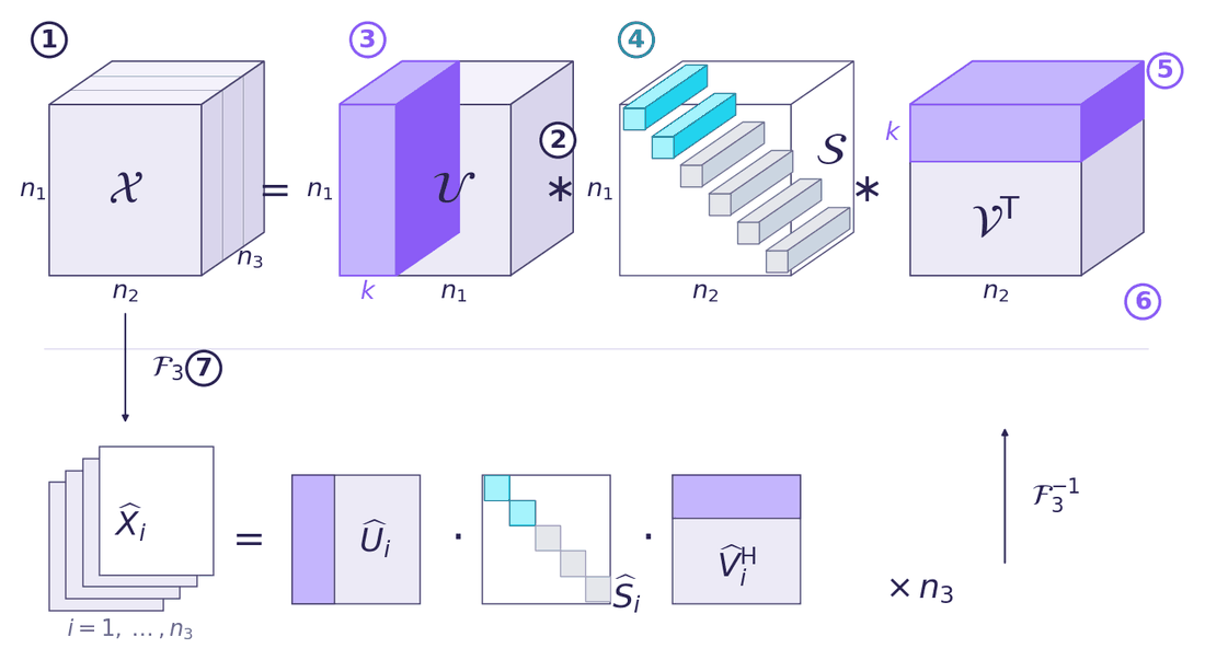
t-SVD, annotated. Violet and cyan mark what a rank-k truncation keeps; the numbers are explained below.

Every shape in the picture means something specific:

1. X is the data tensor, of size n₁×n₂×n₃. The front face is its first frontal slice, and the faint lines behind it are the other slices along the third mode. When I classify images in part four, each image is one lateral slice (n₁×1×n₃), so n₂ is the number of samples.
2. ∗ is the t-product described above, not ordinary matrix multiplication. Every symbol in the picture is a tensor, and each product works along the third mode.
3. U (n₁×n₁×n₃) is orthogonal: U^T ∗ U is the identity tensor. Its lateral slices play the part of the left singular vectors, and the violet block is the first k of them, the basis that a truncated decomposition keeps.
4. S (n₁×n₂×n₃) is f-diagonal. Every frontal slice is a diagonal matrix, so the only non-zero entries are the tubes that run front to back along the diagonal. These singular tubes take the place of singular values. The first k (cyan) are kept and the grey ones are dropped.
5. V^T (n₂×n₂×n₃) is the t-transpose of an orthogonal tensor V: transpose every frontal slice, then reverse the order of slices 2 to n₃. Its first k horizontal slices (violet) are the t-transposes of the first k lateral slices of V. Read column by column and scaled by the singular tubes, they give each sample's coordinates in the kept basis.
6. k is the truncation rank. Keeping only the coloured parts gives X ≈ U_k ∗ S_k ∗ V_k^T, the best Frobenius-norm approximation among tensors of tubal rank at most k.
7. F₃ is a transform along the third mode: the FFT for t-SVD, the DCT for tc-SVD. After it, each frontal slice is factored on its own by an ordinary SVD, X̂_i = Û_i Ŝ_i V̂_i^H for i = 1, …, n₃, with the same truncation in every slice. The inverse transform turns the stacked factors back into U, S and V.

Here is a complete, tested NumPy version. The only subtle part is the second loop: for real input, the slices past the middle must be the complex conjugates of the first half, or the inverse FFT will not come back real.

import numpy as np

def t_product(A, B):
    Af, Bf = np.fft.fft(A, axis=2), np.fft.fft(B, axis=2)
    return np.real(np.fft.ifft(np.einsum("ijk,jlk->ilk", Af, Bf), axis=2))

def t_transpose(A):
    At = np.transpose(A, (1, 0, 2))
    return np.concatenate([At[:, :, :1], At[:, :, :0:-1]], axis=2)

def t_svd(A):
    n1, n2, n3 = A.shape
    Af = np.fft.fft(A, axis=2)
    Uf = np.zeros((n1, n1, n3), complex)
    Sf = np.zeros((n1, n2, n3), complex)
    Vf = np.zeros((n2, n2, n3), complex)
    half = n3 // 2 + 1
    for k in range(half):                      # only half the slices are needed...
        u, s, vh = np.linalg.svd(Af[:, :, k])
        Uf[:, :, k], Vf[:, :, k] = u, vh.conj().T
        Sf[:len(s), :len(s), k] = np.diag(s)
    for k in range(half, n3):                  # ...the rest are complex conjugates
        Uf[:, :, k] = Uf[:, :, n3 - k].conj()
        Sf[:, :, k] = Sf[:, :, n3 - k].conj()
        Vf[:, :, k] = Vf[:, :, n3 - k].conj()
    back = lambda T: np.real(np.fft.ifft(T, axis=2))
    return back(Uf), back(Sf), back(Vf)

A = np.random.rand(6, 5, 4)
U, S, V = t_svd(A)
print(np.allclose(A, t_product(t_product(U, S), t_transpose(V))))   # True

Truncation, the part that matters for learning

As with matrices, you can keep only the first k lateral slices of U and V and the first k diagonal tubes of S. Kilmer and Martin showed that the result is the best Frobenius-norm approximation among tensors of tubal rank at most k, the tensor counterpart of the Eckart-Young theorem. That is what makes t-SVD useful for compression and, as we will see in part four, for classification: a handful of lateral slices of U becomes the feature space you learn in.

The hidden assumption

There is a catch that took me a while to appreciate. The circulant structure encodes an assumption: the third dimension wraps around, so the last slice is treated as the neighbour of the first one. For some data that is harmless. For images and signals it is a bit like assuming the right edge of a photo continues from its left edge.

That observation is where my own contribution starts: tc-SVD, which replaces the wrap-around with a mirror. It is the subject of the next note.

Part of a series based on my M.Sc. thesis, “Big Data Learning with Tensor Representation”, supervised by Dr. Mansoor Rezghi at Tarbiat Modares University.

This note is also available in Persian: read the Persian version.