

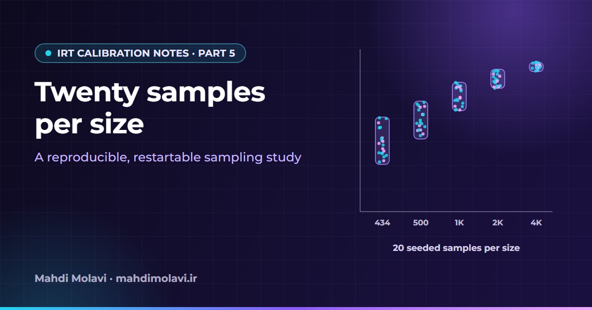
Every experiment so far used one subset per sample size, or a handful. That showed the local estimator's coefficients move with N on fixed questions. It could not say how much of the movement comes from which students happened to be drawn, or whether the pattern holds across tracks and years. That needed a repeated-sampling study, and most of the effort went into the plumbing: deterministic sampling, fits that can be identified and reused, checkpoints that survive interruption, and an output file that keeps different statistical units apart.
The request first mentioned twelve exams. The approved and implemented scope was nine: the three tracks (Mathematics, Experimental Sciences and Humanities) in 1403, 1404 and the original 1405 forms from part 1.
The design
The sampling unit was the student, taken separately for each applicable lesson. A lesson's pool was everyone with a valid score for that lesson and at least one usable response, using the eligibility and response-coding rules from part 2. From each pool:
- target sizes were 434, 500, 1,000, 2,000, 4,000 and 8,000, with duplicate sizes removed;
- each feasible size and lesson got 20 replicates, each one a selection without replacement;
- within a replicate, every larger sample is a prefix of one random permutation, so the 500-person sample contains the 434-person sample, and so on upward;
- a size larger than the pool was skipped and recorded as skipped, never filled by repeating people;
- each lesson also got one fit on its full pool, used as a reference point;
- every main fit used training seed 42, and a separate control refitted the first base subset at seeds 42 to 46 with its people held fixed.
Nesting makes the size comparisons paired: replicate r at N = 4,000 differs from replicate r at N = 434 only by the people added. A student can appear in several replicates, since each draws its own permutation, but never twice inside one sample.
The full-pool fit is a reference, never the true parameter value. With the narrow prior from part 3, it is simply the estimate at the largest N available.
The separate curriculum track inside Humanities had small populations, so its two subjects got their own common base sizes: 226 for Arabic and 221 for history/geography. Its Arabic lesson identifier changed between years, so a comparable-subject mapping allowed comparisons across years while keeping the original identifiers. That curriculum stayed apart from standard Humanities throughout. In total there were 52 lesson-year groups: 48 standard-track groups and four applicable groups in the separate curriculum. A stale lesson row with no active lesson statistics was not counted as an extra subject.
A deterministic sampling recipe
The sample for a given exam, lesson and replicate had to be identical on every run, whatever order the jobs ran in. NumPy's SeedSequence does this from a fixed list of integers. An illustrative sketch in generic form (the seed material matches the study; the generator, hash and dtype choices are mine):
import hashlib
import numpy as np

def replicate_permutation(pool, exam_id, lesson_key, replicate):
    # pool: anonymized student indices in a fixed, canonical order
    ss = np.random.SeedSequence([STUDY_CONSTANT, exam_id, lesson_key, replicate])
    return np.random.default_rng(ss).permutation(pool)

def nested_samples(permutation, sizes):
    for n in sorted(set(sizes)):
        if n > len(permutation):
            yield n, None                 # recorded as Skipped, never padded
        else:
            yield n, permutation[:n]      # prefix: smaller samples nest in larger ones

def fit_key(lesson, n, selected, training_seed):
    ids = np.unique(selected)             # sorted and unique
    fingerprint = hashlib.sha256(ids.astype("<i8").tobytes()).hexdigest()
    return (lesson, n, fingerprint, training_seed)
The study constant looks like a date, but it is one fixed number that never changes between runs. Because the replicate index is part of the seed material, replicate 7 does not depend on whether replicates 1 to 6 ran first. Any recipe like this also needs the pool in a stable order before permuting, or the same seed will pick different people.
The second half of the recipe is identity. After selection, the sorted, unique array of selected student indices (the anonymous per-lesson indices from part 2) is hashed into a population fingerprint, and the fit key combines the lesson, N, that fingerprint and the training seed. Two requests with the same key would fit the same people with the same seed, so the second can reuse the first fit's result. Reuse saves computation. It adds no evidence, and the accounting has to show that.
Counting runs honestly
| Accounting category | Count |
|---|---|
| Designed requested executions, including unsupported sizes | 6,632 |
| Successful executable requests | 4,852 |
| Distinct input/seed fits | 4,760 |
| Requests reusing an identical input/seed fit | 92 |
| Unsupported size/lesson combinations | 89 |
| Requested repeats in those unsupported combinations | 1,780 |
| Complete 20-repeat sample groups | 227 |
| Final failed / pending executions | 0 / 0 |
The 4,852 successful requests are 4,540 sample records (227 complete groups of 20), 52 full-pool records and 260 optimizer-control records (52 lessons at five seeds). The 89 unsupported combinations account for 1,780 requested repeats, and 4,852 plus 1,780 gives the designed 6,632. Of the successful requests, 92 resolved to an input and seed that had already been fitted, which leaves 4,760 distinct fits. I did not count reused fits as independent new evidence.
The run was interrupted and resumed along the way. The saved final segment reports 2,162 fits resumed from checkpoints and 2,598 newly completed ones, which again sums to 4,760. Its elapsed time of about 12,042 seconds belongs to that resumed segment and is not the end-to-end duration of the study.
Making a long run restartable
Thousands of 2,000-epoch fits on CPU take hours, and this work was interrupted. Restarting everything would have thrown away finished computation, so the run resumes from a frozen manifest: the request snapshot, the sampling recipe, and hashes of both the estimator source files and the private input snapshots. Each completed fit writes its own checkpoint, a small JSON summary with versions and provenance plus a NumPy archive holding the item coefficients and the private ability arrays. A separate progress record keeps explicit success, failure and pending counts, and the scheduler picks up whichever fit keys have no checkpoint yet.
Checkpoints are written atomically: write a temporary file, then rename it over the target. On Windows that rename could fail with a PermissionError because the file was briefly locked, even though the fit itself had succeeded, so the rename is retried instead of discarding a finished fit. An illustrative version:
import json, os, time
from pathlib import Path

def save_checkpoint(path: Path, summary: dict, attempts: int = 10) -> None:
    tmp = path.with_name(path.name + ".tmp")
    tmp.write_text(json.dumps(summary), encoding="utf-8")
    for attempt in range(attempts):
        try:
            os.replace(tmp, path)          # atomic on the same volume
            return
        except PermissionError:            # file briefly locked; the fit is fine
            time.sleep(0.2 * (attempt + 1))
    raise RuntimeError(f"could not publish checkpoint {path.name}")
Environment details mattered as much. Persian text broke logging in hidden worker processes whose console encoding could not represent it, and preparation could stop over what was only a logging issue. Running Python in UTF-8 mode (-X utf8) and writing every file as UTF-8 fixed it.
Execution used four worker processes with one computational thread each. The research wrapper set the thread count explicitly, since passing a cores argument to the trainer is no substitute for that control. An illustrative generic version:
import os
for var in ("OMP_NUM_THREADS", "MKL_NUM_THREADS", "OPENBLAS_NUM_THREADS"):
    os.environ[var] = "1"                  # before importing numpy or torch

import torch
torch.set_num_threads(1)
Resumed fits had to be comparable to the earlier ones, so the run verified the SHA-256 hashes of the estimator sources and the library versions before mixing results. The retained environment was Python 3.13, PyTorch 2.7.1 (CPU build), NumPy 2.2.6, pandas 2.3.1, Pyro 1.9.1 and SciPy 1.16.1. A pilot that fitted identical inputs with an identical seed found a maximum parameter difference of zero. That speaks for this research runtime only; the deployed service's seed behavior was never established as identical.
Preparation assertions stopped several early attempts, and I treated each failed gate as a correction to the inputs so that a partial dataset could not pass as a finished study. Exact reruns depend on the frozen local inputs, because a new live extraction can differ as requests, responses and applicability metadata change. The private snapshots and checkpoints stay unpublished, pseudonymized or not.
One CSV, several kinds of row
The main output is one CSV with a RecordType column that keeps different statistical units apart:
- Sample, Full and OptimizerControl: one row per execution;
- SizeSummary: statistics across the repeated executions of one size and lesson;
- ItemStability: one content item's variability across samples;
- SizeComparison: paired changes between a target N and the base N;
- OptimizerSummary: changes across training seeds on a fixed subset;
- CrossExamComparison: descriptive comparisons for a matching course and N;
- Skipped, with explicit failure and pending handling, plus request snapshots, configuration, provenance and execution accounting.
Each fit row summarizes the mean, median, minimum, maximum and SD of a, b, θ and the fixed Lambda, with context such as pool size, actual and requested N, response counts, correct and seen-blank rates, sample raw-score summaries, seeds and elapsed time.
The column that needs the most care is SD, because its meaning depends on the record type. In a SizeSummary row with the across-repeat statistic set to SD, the value in the discrimination-mean column is the SD of 20 lesson-level means. It is not the within-lesson spread of item a values.
The statistics
For each lesson and each larger feasible N, the comparison used the intersection of items present in every base/target pair. Without that, a changing set of fitted items could look like a change in coefficients. For each parameter and replicate r:
delta_r = mean coefficient at target N on the common questions
        - mean coefficient at base N on those same questions
The twenty deltas went through a paired t-test and a two-sided Wilcoxon signed-rank check (with zero_method='pratt'), after rounding differences to 12 decimals so floating-point noise could not turn an exact tie into a tiny nonzero difference. All-zero and nonzero-constant differences got explicit handling, and each comparison recorded a 95% interval for the paired mean difference. An illustrative sketch of one comparison:
from scipy import stats
import numpy as np

d = np.round(target_means - base_means, 12)      # 20 paired differences
if np.all(d == 0) or np.ptp(d) == 0:
    record_degenerate(d)                         # all-zero or nonzero-constant
else:
    t = stats.ttest_rel(target_means, base_means)
    ci = t.confidence_interval(0.95)             # not multiplicity-adjusted
    w = stats.wilcoxon(d, zero_method="pratt")   # two-sided

# later, per test family, across within-exam size contrasts for a and b:
q_t = stats.false_discovery_control(t_pvalues, method="bh")
q_w = stats.false_discovery_control(w_pvalues, method="bh")
Benjamini-Hochberg adjustment was applied separately to the t-test p-values and the Wilcoxon p-values, across the within-exam size contrasts for both a and b, with q < 0.05 as the threshold. Where the two families disagreed, the disagreement was flagged. The individual difference intervals were not adjusted for multiplicity.
The 2.5th and 97.5th percentiles across the 20 samples are reported as sample-variability ranges: how much a lesson's result moved across repeated selections from one frozen pool. I did not call them 95% confidence intervals for true item coefficients, and with only 20 repetitions the tail percentiles are coarse summaries in any case.
What the study found
The results I am comfortable quoting, all from the local narrow-prior estimator on these pools:
- Across the feasible 500-person groups, the median range of the 20 lesson-mean discrimination values was about 0.0345.
- The largest displayed 500-person range was Humanities Economics in 1404, where mean a varied from about 0.4861 to 0.6327.
- For Mathematics-track mathematics in 1403, mean a went from 0.5882 at N = 434 to 1.0881 at N = 4,000, and the average per-fit maximum a from 0.8795 to 1.4862. Over the same change, the samples' mean raw score stayed at about 15.7832 versus 15.7701, and the raw-score SD at about 15.4174 versus 15.5043.
- There were 175 size contrasts for discrimination. All 175 had positive mean changes, and both adjusted test families flagged all of them.
- There were 175 difficulty contrasts: 172 positive changes and three negative. The t-test family flagged 173 and the Wilcoxon family flagged 175, so two decisions disagreed.
- Across the 52 optimizer controls, the median SD of the lesson-mean discrimination across five seeds was about 0.00340, and the median across-seed range about 0.00855.
The 1403 mathematics row is the one I keep coming back to. The students in the larger samples scored the same on average with the same spread, and the estimated mean discrimination nearly doubled. That echoes the pattern of part 3's fixed-question result on a different lesson, this time with twenty nested replicates instead of one subset per size.
What the tests do not say
The tests concern repeated selections from one frozen response pool under the implemented estimator. They do not establish true item parameters, predict the effect of a future recruitment policy, or rank the question quality of different years. With shared data and many contrasts, the analysis is an exploratory diagnostic and no substitute for a dedicated psychometric validation design. A larger a, even a statistically detectable one, does not mean an unchanged question became educationally better.
Sampling fractions matter too. Drawing 500 people from a pool of 521 produces almost identical samples, unlike drawing 500 from several thousand. Near-census repetition naturally shows little selection variation, and zero variation at a full-pool size is not evidence that the coefficients are unbiased or valid outside this pool.
A fixed training seed makes a given input reproducible, but it does not give identical stochastic trajectories across different input sizes. The five-seed control ran on one fixed subset per lesson (the first base subset, not the 500-person samples) and was not crossed with every sample. On its face that spread is small next to the size changes above, but subtracting its variance from the sampling variance to claim a precise decomposition would overstate what it measured.
The acceptance checks covered mappings, unique student/content pairs, curriculum membership, exact sample sizes without replacement, nesting, seeds, finite parameters, unchanged hashes, compatible versions and explicit complete, partial, skipped, failed and pending counts. Passing them makes the study reproducible under its frozen inputs and recorded versions. It does not establish unidimensionality, local independence, invariance or substantive validity.
Part 6 turns to the comparison that came next: lessons across years at equal sample size on replacement current-year forms, a data-coverage bug in those forms, three ways of charting the results, and why none of that amounts to equating.
This note is also available in Persian: read the Persian version.