

With the population defined, the next suspect was the estimator. I opened the model, training and configuration files of the vendored py-irt copy and wrote down every setting the main study used. Most of them were what you would expect. The priors on the item parameters were the exception, and the mode they belonged to was named vague.
The settings
These are the values read from the local source and the research wrapper, as used in the main study:
| Setting | Main-study value |
|---|---|
| Model | Vendored TwoParamLog, a 2PL |
| Prior mode | vague |
| Ability prior | Normal, mean 0, standard deviation 1 |
| Difficulty prior | Normal, mean 0, standard deviation 0.1 |
| Discrimination prior | Normal, mean 0, standard deviation 0.1 |
| Inference | Stochastic variational inference, Trace_ELBO |
| Optimizer | Adam with exponential learning-rate decay |
| Initial learning rate | 0.1 |
| Decay factor | 0.9999 per training step |
| Training length | 2,000 epochs |
| Export | best_params, from the lowest observed training loss |
| Main training seed | 42, set explicitly by the research wrapper |
| Execution | CPU; four processes, one computational thread per process |
| Lambda output | Fixed 0.25 |
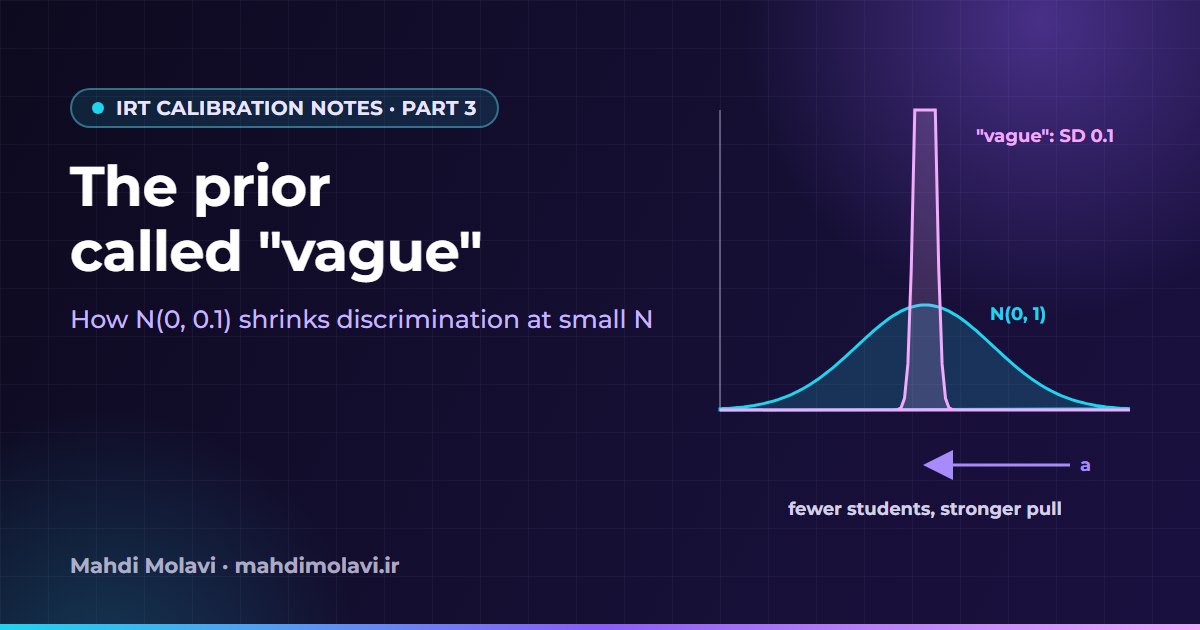
The ability prior, N(0, 1), is a standard choice. The item priors are the interesting rows. The 0.1 in them is a standard deviation, so the variance is 0.01. A normal distribution with SD 0.1 puts about 95% of its mass between −0.2 and 0.2. For a discrimination parameter, where values around 1 and above are ordinary, that is a strongly concentrated prior, whatever the configuration calls it.
What the prior costs
Ignoring constants, the negative log-density of that discrimination prior is
a^2 / (2 * 0.1^2) = 50 * a^2
and the same expression applies to difficulty. At a = 1 the term is 50, and at a = 2 it is 200. Every observed response adds a likelihood term that pulls toward whatever slope the data support. When a question has few responses, the pull of the prior toward zero carries more weight relative to that evidence. With many responses, the likelihood can support values farther from zero.
I use that expression to explain shrinkage. It cannot be used to compute the exported coefficient. The fit is variational: the prior term sits inside an expected objective together with the likelihood and the entropy of the guide, the approximating distribution that the optimizer adjusts. The Pyro SVI tutorial explains the split between model, guide and ELBO well if you have not met it.
A few details of the guide are worth keeping in mind, because they are easy to misdescribe:
- The ability location starts at zero and its scale at one.
- The difficulty location starts at zero and its guide scale at 10.
- The discrimination location starts at one and is constrained to be positive; its guide scale starts at 1e-6.
The positive constraint is on the guide's location. The generative prior on discrimination is still an ordinary Normal, so calling it a lognormal or a truncated Normal prior would describe a different model.
Then there is the export. best_params is the parameter set at the lowest training loss the run observed. It is a point estimate from a stochastic procedure. It does not prove convergence, and it carries no posterior uncertainty interval. Reproducibility also needed explicit control: the research wrapper set the seed and the thread counts itself, because merely passing a cores argument is not a substitute for that control. I did not establish that the production service's implicit seed behavior or its exact runtime matched the research runtime.
Same questions, different N
An argument about priors is cheap. The experiment that convinced me held the questions and the source responses fixed and changed only the number of students. I took the 30 mathematics questions of the 1403 Experimental Sciences archive exam, where 9,099 students had usable responses in that extraction, and drew subsets of different sizes from that same frozen source. These values come from the later fresh controlled run, not from the earlier exploratory fits:
| N | Correct-response rate | Mean a | Maximum a | Mean b | SD of each person's correct-response proportion |
|---|---|---|---|---|---|
| 434 | 9.073% | 0.7665 | 0.9043 | 0.2767 | 0.12395 |
| 1,000 | 9.037% | 0.9953 | 1.1387 | 0.5168 | 0.12329 |
| 4,000 | 9.074% | 1.3594 | 1.5826 | 1.1233 | 0.12004 |
| 9,099 | 8.753% | 1.4986 | 1.7853 | 1.5166 | 0.11790 |
The questions are the same in every row. The correct-response rate stays near 9%, and the spread of the students' observed correct-response proportions does not grow with N; it shrinks slightly. Yet the mean a roughly doubles between 434 and 9,099 students, and the maximum a goes from about 0.90 to about 1.79.
My interpretation is that this is an interaction between the estimator and the sample size, and it is much stronger evidence than comparing maxima across unrelated exams. The limits are real, though. This early table used one selected subset per smaller size, so it shows a direction and a rough size for one lesson. It does not give the size of the effect in every lesson or population. Part 5 repeats the experiment with twenty samples per size over nine exams.
Widening one prior
If the narrow prior drives the pattern, loosening it on unchanged data should move the estimates. I took the 523-person mathematics response set of the current Experimental Sciences exam and, in memory, widened only the discrimination prior's SD from 0.1 to 0.5. The source files were not edited. The fresh default fit had a maximum a of about 0.934. The sensitivity fit had a maximum of about 2.637 and a mean a of about 1.962.
That is a large move from one setting, and it is evidence that the estimate depends strongly on the prior. It does not show that 0.5 is the right prior, that the larger values are the true ones, or that production should switch immediately. Earlier exploratory reports contain nearby values that differ from these, for example different maxima for a 523-person archive subset. Those were separate draws and refits, and I keep this named fresh control as the single coherent example.
Can 434 students support high discrimination?
Real questions have unknown true parameters, so real data alone cannot separate "these questions have low discrimination" from "this estimator returns low discrimination at this size". A simulation can. I generated three independent binary response matrices, each with 434 students and 30 questions:
theta ~ Normal(0, 1)
true discrimination values: 2.0 to 3.5, mean 2.75
true difficulty values: -1.5 to +1.5
Y ~ Bernoulli(sigmoid(a * (theta - b)))
These are synthetic matrices, not authored educational questions. I fitted each with the current code and with a small reference estimator by marginal maximum likelihood (MML). The reference estimator did not receive the true abilities.
| Simulation | True mean a | Current-code mean a | Reference MML mean a | Current-code a RMSE | Reference MML a RMSE |
|---|---|---|---|---|---|
| 1 | 2.750 | 0.676 | 2.593 | 2.116 | 0.371 |
| 2 | 2.750 | 0.678 | 2.664 | 2.115 | 0.386 |
| 3 | 2.750 | 0.677 | 2.838 | 2.112 | 0.307 |
The reference estimator was a small research comparator built for this check. It integrated over an N(0, 1) ability distribution with Gauss-Hermite quadrature and optimized log(a) and b with L-BFGS-B. It makes no claim to be a full testing program's machinery. Raising its quadrature from 121 to 181 points on the first dataset changed the maximum a by about 0.00017, so the grid was not driving its results. It is also a separate implementation from the GIRTH evaluation in part 4.
The current code returned a mean a of about 0.68 on data generated with a mean of 2.75, in all three runs, and its error was more than five times that of the comparator. One question makes this concrete. Synthetic question 29 in the first simulation had a true a of 2.4138. The current code estimated 0.7014, and the MML comparator estimated 2.4601. A bootstrap of the comparator over the students gave an approximate 95% interval of [2.0507, 3.1238], and all 200 bootstrap fits converged.
What this supports: N = 434 does not impose a ceiling that forces discrimination below one. Under favorable conditions, with a known model and generated data, high discrimination can be recovered at that size. What it does not support: that the real production questions have a true a near 2.75, or that 434 students guarantee adequate precision for every question.
Why "200 students is enough" did not answer the question
The rule of thumb from part 1 came back at this point, because on its face 434 students passes it. No sample-size cutoff guarantees accurate coefficients for every model and response pattern. The N that matters is often the number of usable responses per question, which can differ from registrations or official attendance, as part 2 showed. Precision depends on the model, the estimator, the prior, the difficulty and discrimination of the question, how well the ability range is covered, missingness and the policy for omitted responses, and how accurate the decision needs to be.
Published guidance exists. The ETS introduction to IRT discusses approximate sample sizes, with qualifications that tend to get lost when the guidance turns into a slogan. For this pipeline, the same-question size experiment and the simulation told me more than any generic threshold could. Under the local code, 434 students on the fixed questions gave a mean a of 0.7665, against 1.4986 for the full pool of 9,099.
Difficulty moved too. In that controlled fixed-question table, the mean b rose from about 0.277 to 1.517 between 434 and 9,099 students. The question texts did not become harder as more people took them, so that drift belongs to the estimation, and it is a warning for anyone who compares b values across exams of different sizes from this pipeline.
Where this leaves the explanation
I can now state a narrower claim with some confidence. On fixed questions, the coefficients of the local narrow-prior estimator changed strongly with N, and the prior sensitivity check and the simulation both point to prior and estimation effects. That supports an explanation for this implementation. It does not show that the prior alone explains every difference in the production tables, and it does not imply that every Bayesian estimator would behave this way. It certainly does not mean that more students make a question more discriminating.
The obvious next question was whether a different estimator would behave better. Part 4 tries two: a hierarchical prior inside the same library, which brought its own orientation problems, and marginal maximum likelihood through GIRTH.
This note is also available in Persian: read the Persian version.