

Three exams from the current year, one for each track, came back from calibration with a maximum estimated discrimination well below what the archive showed for the same tracks. The data belonged to an online exam platform whose analytics I was working on, and the question that reached me was short: are the new questions worse? Read at face value, the result table said yes. The new forms seemed to separate stronger and weaker students less sharply than the forms from two years earlier.
The first thing I noticed was attendance. The archive exams I was comparing against had been taken by far more people:
| Track | Current exam (1405), official attendance | Archive exam (1403), official attendance |
|---|---|---|
| Mathematics | 434 | 6,342 |
| Experimental Sciences | 521 | 9,222 |
| Humanities | 1,134 | 8,648 |
A gap of roughly 8 to 18 times in attendance next to a drop in discrimination is a coincidence I did not want to accept or dismiss without looking. Several explanations fit the summary. The new questions might be weaker, the new cohorts might vary less, the samples might be too small, or the estimator might respond to sample size by itself. A familiar rule of thumb was also in the room: more than 200 students is enough for calibration. If that rule held, sample size was off the list for all three exams. Each explanation predicts something you can check, and checking them took longer than I expected and changed how I read the original metric.
What this series covers
This series is my record of that investigation. I wrote it for backend and data engineers, for people who run assessment systems, and for developers who are curious about psychometrics. Each part takes one layer of the problem:
- Part 1, this one: the puzzle, a short refresher on the 2PL model, two names in the code that pointed the wrong way, and what reading the code did and did not prove.
- Part 2: who entered the calibration. Attendance, usable responses and stored abilities are different counts, and the response coding decides what a zero means.
- Part 3: a prior labeled "vague" that is quite narrow, an experiment where the questions stayed fixed and only N changed, and a simulation that asks whether 434 students can support high discrimination at all.
- Part 4: two other estimators, a hierarchical prior and marginal maximum likelihood through the GIRTH library, with their own failure modes.
- Part 5: a repeated-sampling study over nine exams, twenty samples per size, and the engineering that made it restartable and reproducible.
- Part 6: equal-N comparisons across years, how the results were reported, and why equal N is not equating.
Throughout, I keep observations, interpretations and proposals apart, and I say where a result stops applying. The numbers come from several phases of the work, with different extractions and different populations. I will not merge them, even when two of them look close enough to tell a neater story.
The model in a few lines
The estimator behind these coefficients fits a two-parameter logistic model, the 2PL. For student s and question i:
P(correct response by student s to item i) = sigmoid(a_i * (theta_s - b_i))

sigmoid(x) = 1 / (1 + exp(-x))
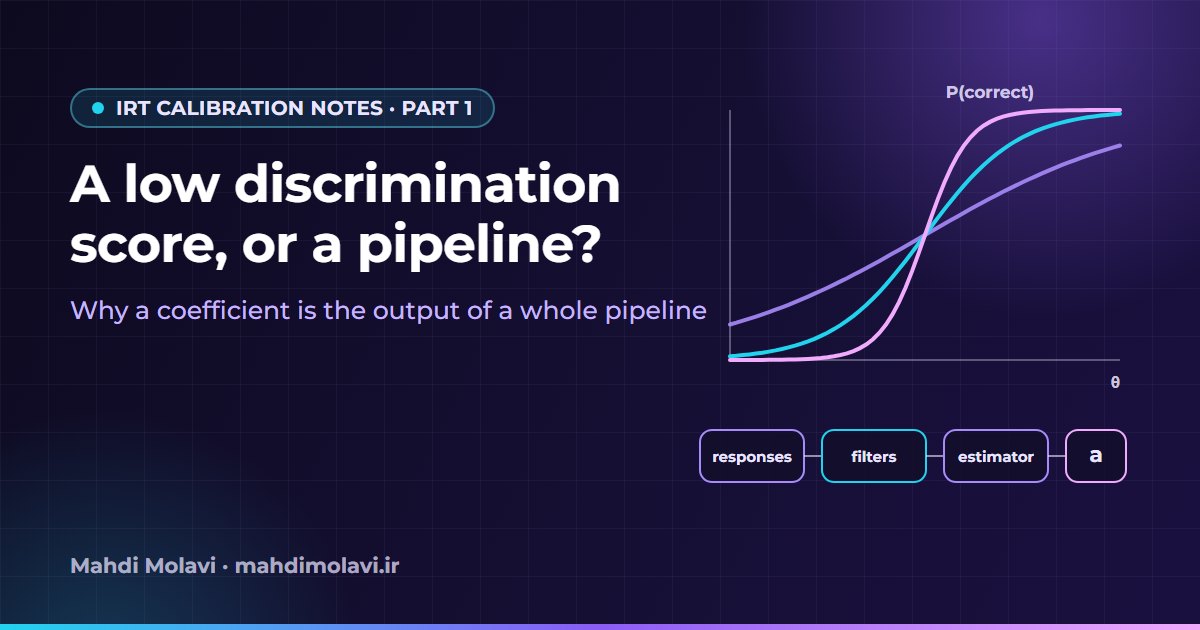
θ is the student's latent ability. Nobody observes it directly; the model estimates it along with the item parameters. b is the difficulty, and in this parameterization it is the ability at which the modeled chance of a correct answer is 0.5. a is the discrimination, the steepness of the curve around b. A question with a large positive a separates students whose abilities lie near its difficulty quite sharply, while a question with a small a gives similar chances to students who are far apart.
Two cautions apply from the start. A difficult question is not automatically a bad one, and a high-discrimination question is not automatically right for every population or content objective. The metric under suspicion, the largest a in an exam, carries both cautions with it. I wrote about how the same parameters drive item selection in Backend Notes 2, on adaptive testing with IRT. This series is about where the parameters come from.
Two names that pointed the wrong way
The result tables carry a column called Lambda, and every row I looked at said 0.25. The service function that runs the estimation has "3pl" in its name. Together those two facts suggest a three-parameter model with an estimated guessing floor. When I read the function, it called the library's 2PL class. Lambda appears nowhere in the fitted response function; the output pipelines write it as a fixed value. A model that really estimated guessing would fit a lower asymptote c:
P = c + (1 - c) * sigmoid(a * (theta - b))
That is a different response function from the one fitted here. I put this first because it is the cheapest mistake in the whole story and the most embarrassing one to publish. A report that says the platform estimates a 3PL invites comparisons with 3PL guidance that do not apply. For the rest of the series every coefficient is a 2PL coefficient, and Lambda is a stored constant.
Did the students vary less?
One explanation on the table was that the new cohorts were more alike. Discrimination needs contrast between students, the argument went, so a homogeneous group produces flat curves. The official lesson statistics allowed a first check. In the main mathematics lesson of each track, raw percentage scores and the stored maximum discrimination looked like this:
| Track | Current mean / SD of raw percentage score | Archive mean / SD | Stored mathematics maximum a, current / archive |
|---|---|---|---|
| Mathematics | 22.10 / 16.62 | 15.80 / 15.56 | about 0.90 / 1.54 |
| Experimental Sciences | 8.60 / 14.47 | 5.10 / 11.13 | about 0.96 / 1.73 |
| Humanities | 9.40 / 14.02 | 5.20 / 11.70 | about 1.22 / 1.72 |
In all three tracks the new exam had the larger raw-score spread, and in all three its stored maximum discrimination was lower. The simple version of the homogeneity story predicts the opposite. The table has limits, though, and I want them on the record. These are lesson-specific stored statistics, so the maxima here are not maxima across every lesson and sublesson row. Raw-score SD describes observed scores, and the SD of latent ability is a different quantity. The old and new exams also had different questions. What the table does is remove one easy explanation. It leaves the cause unidentified.
Three kinds of variation
Before going further, it helps to separate three quantities that all get called "variation" in conversation. They answer different questions, and later parts measure them with different tools.
| Quantity | What varies | What it answers |
|---|---|---|
| Between-item distribution | Different questions in one lesson and year | How different are the fitted coefficients of the questions? |
| Sampling variability | Students selected from the same frozen response pool | How much does the answer change when the calibration sample changes? |
| Training randomness | The training seed, with exactly the same response subset | How much does stochastic fitting change the answer? |
A wide spread of coefficients across one exam's questions tells you nothing about how stable any single coefficient is, and a coefficient that barely moves under resampling may still move with the optimizer's seed. Part 5 measures the second and third quantities. The histograms and boxplots in part 6 show the first, and a narrow box there is not a narrow confidence interval for any question.
Reading the code
The first practical question was whether two codebases on the platform calculated the same parameters with the same logic and settings. One of them served adaptive tests. In the feature I inspected, it read existing item parameters from its own item tables, and I found no equivalent end-to-end calibration entry point there. Nobody supplied another one for me to check. The second codebase was the one doing calibration.
Both carried a vendored copy of py-irt, the open-source IRT library built on Pyro. I compared four of its files by SHA-256: the 2PL model, the dataset class, the training loop and the configuration. All four were byte-identical across the two repositories.
Matching hashes prove exactly one thing, which is that those four files match. They say nothing about which responses each service selects, how it groups them, what runtime settings it uses, or whether it runs a calibration at all. Here, I found no calibration entry point in the inspected code of one of the two services, so the match was true and close to irrelevant. The hashes cannot carry the claim that both applications calibrate identically.
Inside the calibrating codebase there were two code paths into the same estimator. The first read per-question response records from the analytics warehouse's response fact table, joined them through the active analysis request and the question dimensions, excluded responses with answer status 5 (unseen), grouped them by assessment lesson and called the estimator. The second was built around assessment-run results. It fetched responses and compact answer sheets through stored procedures, merged them by exam, user and content, gave the answer-sheet responses precedence, mapped each selected choice against a cached answer key, grouped by assessment lesson and lesson, called the same 2PL classes and wrote its own result models. In generic form, the estimator call looked like this:
trainer = TwoParamLog.train(data, device="cpu", epochs=2000)
params = trainer.best_params
So the model class and the training call were shared, and the inputs were prepared differently. The answer-sheet path can materialize a blank entry for a known question as an explicit response row, and such a row is not automatically equivalent to the unseen status in the fact table. One count in its output has a name that suggests "students who answered". It counts the users present in the merged input, and its name alone does not prove that each of them chose a substantive answer.
The two paths fed different result tables. The coefficients people were worried about lived in the result table for assessment runs, while a separate content-bank table held another calibration. Treating those two branches as one was an early wrong turn, and I corrected it by following the run-level table and its run and lesson keys. When I later built research jobs, they imported the estimator classes directly and never called the write-capable HTTP endpoint.
This comparison has a firm boundary. I compared current source code, which is a different thing from a historical deployment audit. The saved research results do not establish the stored-procedure implementations, the deployed versions, the exact production input snapshots or past configuration states. I therefore cannot say that every stored run used the input rules of the path I later used for research, and I do not say it.
A coefficient is the output of a pipeline
By this point the original question had changed shape. "Are the new questions worse?" treats a stored a value as a property of a question. In practice it is the end of a chain of decisions: who was selected, how their answers were coded, which model and prior were fitted, how the optimizer ran and when it stopped, and how the numbers were aggregated for a report. Until each link has been examined, a difference in the output cannot be attributed to question quality.
Seeing it this way also gave me a work plan. Each stage could be checked on its own terms: the population against the database, the model against its source, and the estimator against controlled experiments in which I knew what ought to happen. Some of those checks removed explanations that had seemed obvious, and a couple uncovered data problems that a better model would not have fixed. The rest of the series follows that order.
Part 2 starts with the population: six legitimate counts of "students" for a single lesson, and the coding rule that decides what an unanswered question means.
This note is also available in Persian: read the Persian version.