

Take the current Experimental Sciences exam and its mathematics lesson. In the first six-exam investigation I had four student counts for it: 521, 530, 522 and 523. Every one of them was correct. They counted different things, and the comparison in part 1, which used official attendance, depended on a number the estimator never saw.
This part is about the population: which students and which responses entered the calibration, and what each response was allowed to mean. Most of it is data engineering, with no IRT in it. It still shaped what the coefficients meant.
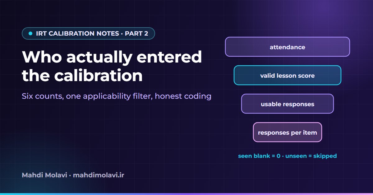
Six counts, all legitimate
For a single exam and lesson, at least six quantities can be called "the number of students":
- Official attendance for the exam.
- Students with a general student-statistics record.
- Students with a valid score for that particular lesson.
- Students with at least one usable response in that lesson.
- Students with an ability stored by an earlier calibration.
- The effective number of observed responses to one particular question.
For that Experimental Sciences exam, the four I had were 521 official attendees, 530 general student-statistics records, 522 students in the previously stored mathematics IRT output, and 523 students in a fresh extraction of usable mathematics responses. None of these is interchangeable with another. Attendance came from an exam-level summary table and the lesson figures from a lesson-level summary, both for the relevant active analysis request. Those aggregates are useful for reporting, and I still did not let them stand in for the eligibility checks at the level of individual responses.
The last count on the list matters most for the estimator. A question's coefficient is fitted from the students who were shown that question, and part 3 comes back to this when it looks at the "200 students is enough" rule. Attendance is simply the number that is easiest to find.
Even one definition can move between snapshots. An early snapshot reported 1,132 Humanities attendees, and a later recheck gave 1,134. The final nine-exam study froze the later value. I treat that as a version and provenance issue, and I recorded which snapshot every number came from instead of blending them.
Requests and identity
On this platform each response row in the analytics warehouse belongs to an analysis request. The research selection path joined the tables in this order, described here by role:
per-question response fact rows
    -> analysis request (active requests only)
    -> assessment question
    -> question
    -> content item id
I accepted only completed analysis requests. The request identity was recorded with each extraction and rechecked later, so a rerun could confirm it was reading the same analysis and not a newer one. This sounds like bookkeeping, and it is. It is also what later let me say which responses a given number came from.
Which lessons applied
The existence of a response row did not prove that a lesson applied to the student. To count a student in a lesson, I required a non-null raw score in the lesson statistics for the same request, the same student and the applicable lesson.
Humanities shows why. Alongside the standard Humanities lessons there is a separate curriculum track with its own subjects. In an earlier archive extraction, that track's history and geography lesson had 8,148 users with seen rows before the applicability filter and 328 after it. Its Arabic lesson went from 8,335 to 275. Response rows existed for thousands of students who were outside that course. When the unsuitable input was fitted, it produced extreme discrimination estimates, and those estimates did not remain in the corrected results from the independent estimator in part 4.
The raw score had one job in this pipeline: deciding applicability, plus some reporting. It was never an IRT observation. The fitted observations were the binary response statuses described in the next section. I mention it because a column called raw score sitting next to response data invites someone to use it as an input, and that would be a different model.
What a zero means
The response fact table stores an answer status for each student and question. The research treatment was:
| Source response | Research treatment |
|---|---|
| Status 1 | Observed correct response, Y = 1 |
| Status 2, 3 or 4 | Observed non-correct response, Y = 0 |
| Status 4: seen but left blank | Included as zero |
| Status 5: unseen | Excluded from the likelihood |
| No response record | Not invented, and not filled in as an observed zero |
People often summarize this as "only the questions the student answered", and the shorthand is wrong. Seen blanks stay in the data as zeros: the student saw the question and gave no correct answer. Unseen questions are left out, because a question the student never saw carries no evidence about their ability. And where no record exists, nothing is added. A pipeline that turns every missing cell into a zero would treat absence as failure, and the fitted difficulty and discrimination would absorb that choice with no visible sign.
A made-up student shows the size of the choice. Suppose a form has 30 questions and the student is shown 20 of them, answers 8 correctly, gets 8 wrong and leaves 4 blank. Under the research coding that student contributes 20 observations to the likelihood, 8 ones and 12 zeros, and the 10 unseen questions contribute nothing. Code the unseen questions as wrong and the same student contributes 30 observations with 22 zeros. Their estimated ability drops, and every one of those 10 questions now looks as if a student failed it. Multiply that by a cohort and the item parameters move with it.
These rules describe the research extraction. As part 1 showed, the run-based path rebuilt responses from answer sheets and could create explicit blank rows for known questions. I did not assume that its blanks lined up with this table.
The helper that decides for you
The vendored library builds its dataset from the response rows with a helper that converts every status other than 1 to zero. Pass it unseen rows and they become wrong answers. The same helper drops duplicate student and item pairs. If two copies of a pair disagree, one silently survives, and the helper's internals decide which.
Both behaviors are reasonable defaults for a library and dangerous ones for a pipeline that has not made its own decisions first. So the order in the research jobs was fixed: filter out unseen responses before calling the helper, and check for duplicates before calling it too, so that deduplication never happened by accident. A sketch of that order, with invented column names:
# The library helper maps every status except 1 to 0,
# and keeps one row per (student, item) without telling you which.
rows = rows[rows["status"] != 5]            # unseen: not an observation

dupes = rows.duplicated(["student", "item"], keep=False)
if dupes.any():
    raise ValueError("duplicate student/item pairs; resolve them before fitting")

rows["y"] = (rows["status"] == 1).astype(int)   # 2, 3, 4 (incl. seen blank) -> 0
Part 6 tells a longer version of this story. When the current-year forms were replaced, duplicated copies of responses showed up in large numbers, and the rule became stricter: consistent copies could be collapsed after a canonical mapping, and conflicting copies stopped the run.
Privacy and snapshots
All of this work used real student responses, so a few rules applied throughout. Before any research input snapshot was retained, student identifiers were replaced with anonymous indices assigned per lesson. Exported CSV reports did not contain real student identifiers. Public result packages left out response rows and individual ability vectors. The abilities in the simulation of part 3 were generated values and had nothing to do with student records.
Every query was read-only. I read the source application's write functions to understand what they did, and the research pipeline never called them. The queries ran under READ UNCOMMITTED to reduce contention with the live system. That isolation level avoids taking shared locks, which is why it is gentle on a busy database. It also means a long extraction can read uncommitted rows and rows from different moments, so the result is not a transactionally consistent snapshot of history.
That is why the frozen inputs mattered. Each extraction was saved locally with its request identities and a hash, and every exact rerun read the frozen file instead of querying again. A fresh live extraction can legitimately differ from an older one, because requests, responses and applicability metadata change over time. Stored production coefficients did not always carry enough request provenance to reconstruct their exact inputs, so I keep them apart from fresh refits and do not invent a cause for every discrepancy between the two.
What this changed
The population work changed one set of coefficients directly: the extreme estimates from the separate curriculum track. Its larger effect was to turn "N" from a single number into a definition I could write down: completed and active analysis request, applicable lesson with a valid score, at least one usable response, seen blanks as zeros, unseen excluded, duplicates resolved before the library saw them. With that definition in place, a comparison between two exams at least compares the same kind of thing. Without it, the attendance table in part 1 could not tell me anything about the questions.
Once the population was pinned down, I turned to the estimator itself. Part 3 looks at its prior, which the code calls "vague", and at what happens to the same thirty questions when only the number of students changes.
This note is also available in Persian: read the Persian version.